
Learning objectives / 学习目标
- 对不可分辨单原子经典理想气体构造 \(Z_N\),解释 \(N!\) 与 thermal wavelength,并推出 \(pV=Nk_BT\)、\(U=3Nk_BT/2\)。
- 由独立磁矩的二态配分函数推导 magnetization、Curie susceptibility、internal energy 与 Schottky-like heat capacity。
- 对一维 classical harmonic oscillator 完成 phase-space Gaussian integral,并由 \(Z\) 求 \(U,C_V\) 与均方涨落。
- 从 Gaussian integration 或 generalized equipartition identity 说明每个独立二次项贡献 \(k_BT/2\) 的条件。
- 用 quantum energy spacing、indistinguishability、mode freeze-out 与相互作用解释 equipartition breakdown,而不是把偏差归因于“能量不守恒”。
- 对每个应用执行无量纲性、极限、单位、粒子可分辨性与 dilute classical limit 检查。
Prerequisites / 先修知识
- canonical ensemble、\(Z\) 的对数导数与涨落。
- ideal-gas equation and kinetic interpretation。
- Gaussian integral \(\int_{-\infty}^{\infty}e^{-ax^2}dx=\sqrt{\pi/a}\)。
- 简单磁矩能量 \(E=-\boldsymbol\mu\cdot\mathbf B\) 与谐振子 Hamiltonian。
Scope and conventions / 范围与约定
- 默认 Maxwell–Boltzmann dilute regime:number density \(n\) 满足 \(n\lambda_T^3\ll1\);量子简并留给 Unit 3.7。
- 单原子气体忽略粒子间相互作用和内部自由度,容器体积远大于边界层尺度。
- 顺磁模型是 \(N\) 个固定位置、非相互作用的二态磁矩,磁场沿 \(+z\);用 \(\mathcal M\) 表示总磁矩,避免与粒子质量 \(m\) 混淆。
- 谐振子为一维、classical、平衡、二次 Hamiltonian;相空间积分除以 \(h\) 以无量纲化。
- \(C_V\) 指总系统热容;每粒子或每摩尔结果会显式标注。
Notation and modeling contract / 符号与建模契约
| Symbol | Meaning | SI unit |
|---|---|---|
| \(m\) | particle or oscillator mass | kg |
| \(n=N/V\) | number density | \(\mathrm{m^{-3}}\) |
| \(\lambda_T\) | thermal de Broglie wavelength | m |
| \(Z_N\) | \(N\)-particle canonical partition function | 1 |
| \(\mu_m\) | magnitude of one magnetic moment | \(\mathrm{J\,T^{-1}}\) |
| \(B\) | magnetic flux density along \(+z\) | T |
| \(\mathcal M\) | total magnetic moment along \(z\) | \(\mathrm{J\,T^{-1}}\) |
| \(\chi_B\) | derivative \((\partial\mathcal M/\partial B)_T\) | \(\mathrm{J\,T^{-2}}\) |
| \(C_B\) | heat capacity \((\partial U/\partial T)_{B,N}\) at fixed applied \(B\) | \(\mathrm{J\,K^{-1}}\) |
| \(k_s\) | oscillator spring constant | \(\mathrm{N\,m^{-1}}\) |
| \(\omega\) | oscillator angular frequency \(\sqrt{k_s/m}\) | \(\mathrm{s^{-1}}\) |
| \(x=\beta\mu_mB\) | dimensionless magnetic field | 1 |
| \(f\) | active independent quadratic energy terms per particle or molecule | 1 |
Knowledge 1 — Ideal gas from the partition function / 由配分函数导出理想气体
Knowledge ID: P03-U06-L03-K01
1.1 单粒子相空间积分给出 thermal wavelength
单原子自由粒子的 Hamiltonian 是 \(H_1=\mathbf p^2/(2m)\)。单粒子 canonical partition function 为
\[z_1=\frac{1}{h^3}\int_Vd^3q\int d^3p\, e^{-\beta\mathbf p^2/(2m)}.\]
位置积分给 \(V\),三个 Gaussian 动量积分给 \((2\pi mk_BT)^{3/2}\),因此
\[z_1=\frac{V}{\lambda_T^3}, \qquad \boxed{\lambda_T=\frac{h}{\sqrt{2\pi mk_BT}}}.\]
同种不可分辨经典粒子需要 Gibbs correction:
\[\boxed{Z_N=\frac{1}{N!}\left(\frac{V}{\lambda_T^3}\right)^N}.\]
\(h^{3N}\) 使相空间积分无量纲,\(N!\) 避免把仅交换粒子标签的配置重复计数。这个 classical formula 保留了 \(h\),因为经典连续态计数仍需一个相空间单元;可测经典状态方程最终不依赖 \(h\)。
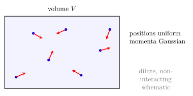
图 1:经典理想气体的相空间权重分离为均匀位置部分和 Maxwell–Gaussian 动量部分;箭长不按比例。
1.2 对数导数恢复 ideal-gas thermodynamics
由 \(F=-k_BT\ln Z_N\) 以及 Stirling approximation,
\[F\approx-Nk_BT\left[\ln\left(\frac{V}{N\lambda_T^3}\right)+1\right].\]
于是
\[p=-\left(\frac{\partial F}{\partial V}\right)_{T,N} =\frac{Nk_BT}{V},\]
\[U=-\frac{\partial\ln Z_N}{\partial\beta} =\frac32Nk_BT, \qquad C_V=\frac32Nk_B.\]
经典有效性参数是 phase-space density:
\[\boxed{n\lambda_T^3\ll1}.\]
当它接近或大于 \(1\),粒子波包重叠,不可忽略 Bose/Fermi statistics。
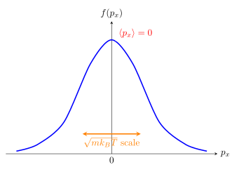
图 2:每个动量分量是中心在零的 Gaussian;对称性给零平均但非零 \(\langle p_x^2\rangle\)。
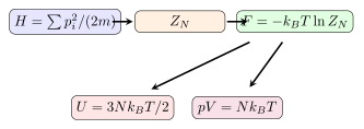
图 3:由 free-particle Hamiltonian 经相空间积分与统计势,同时生成 mechanical equation of state 与 caloric equation。
Worked Example 1 — 一摩尔单原子理想气体的 \(p,U,C_V\)
已知条件: \(n_{mol}=1.000\ \mathrm{mol}\) 单原子稀薄气体,\(T=300.0\ \mathrm K\),\(V=2.460\times10^{-2}\ \mathrm{m^3}\)。
研究对象: 容器内全部气体。
系统边界与参考系: 刚性容器,静止实验室系;平衡且无宏观流动。
模型及理由: 稀薄、单原子、非相互作用,使用 classical ideal-gas partition result;\(N k_B=n_{mol}R\)。
\[p=\frac{n_{mol}RT}{V} =\frac{(1.000)(8.314462618)(300.0)}{2.460\times10^{-2}} =1.01396\times10^5\ \mathrm{Pa}.\]
\[U=\frac32n_{mol}RT =3.74151\times10^3\ \mathrm J,\]
\[C_V=\frac32n_{mol}R =12.4717\ \mathrm{J\,K^{-1}}.\]
有效数字与单位: 由 \(T,V\) 给出四位有效数字;\(p\) 为 Pa,\(U\) 为 J,\(C_V\) 为 \(\mathrm{J\,K^{-1}}\)。
检查与解释: \(pV=2494\ \mathrm J=nRT\),量纲为能量;\(U\) 与 \(V\) 无关是 noninteracting monatomic model 的结论,不适用于致密真实气体或内自由度已激活的分子气体。
Knowledge 2 — Paramagnetism and two-state systems / 顺磁性与二能级系统
Knowledge ID: P03-U06-L03-K02
2.1 二态磁矩的 partition function
每个固定磁矩沿外场 \(\mathbf B=B\hat{\mathbf z}\) 只能取 parallel 或 antiparallel,能量为
\[E_{\uparrow}=-\mu_mB, \qquad E_{\downarrow}=+\mu_mB.\]
单磁矩配分函数及 \(N\) 个独立磁矩的配分函数是
\[z_1=2\cosh x, \qquad Z_N=(2\cosh x)^N, \qquad x=\frac{\mu_mB}{k_BT}.\]
由 \(\mathcal M=-\partial F/\partial B\) 得
\[\boxed{\mathcal M=N\mu_m\tanh x}.\]
弱场高温 \(x\ll1\) 时 \(\tanh x\approx x\),所以
\[\mathcal M\approx\frac{N\mu_m^2}{k_BT}B, \qquad \chi_B=\left(\frac{\partial\mathcal M}{\partial B}\right)_T \approx\frac{N\mu_m^2}{k_BT},\]
即 Curie \(1/T\) law。这里 \(\chi_B\) 是总磁矩对 \(B\) 的导数;若使用体磁化强度与 \(H\) 场,SI susceptibility convention 会不同。
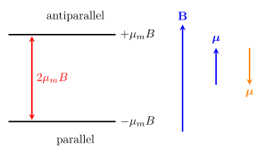
图 4:外场劈裂二态能级;parallel state 能量较低。右侧箭头是取向示意,不按比例。
2.2 饱和磁化与 Schottky-like heat capacity
平均能量与固定外加磁场的热容 \(C_B\equiv(\partial U/\partial T)_{B,N}\) 为
\[U=-N\mu_mB\tanh x,\]
\[\boxed{C_B=Nk_Bx^2\operatorname{sech}^2x}.\]
\(T\to0\) 时磁矩几乎全在低能态,\(\mathcal M\to N\mu_m\) 且 \(C_B\to0\);\(T\to\infty\) 时两态趋于等占据,\(\mathcal M\to0\) 且因能量饱和 \(C_B\to0\),中间出现峰。
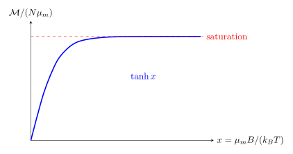
图 5:独立二态磁矩的总磁矩由线性 Curie 区逐渐进入饱和区。
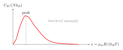
图 6:二能级热容在低温冻结与高温饱和之间出现 Schottky-like peak;横轴随降温增大。
Worked Example 2 — 稀疏独立磁矩的磁化与热容
已知条件: \(N=1.00\times10^{23}\) 个独立磁矩,\(\mu_m=9.27401\times10^{-24}\ \mathrm{J\,T^{-1}}\),\(B=1.00\ \mathrm T\),\(T=5.00\ \mathrm K\)。
研究对象: 固定位置的全部磁矩;忽略晶格热容。
系统边界与方向: 与热库接触,外场沿 \(+z\);\(\mathcal M>0\) 表示沿场。
模型及理由: 非相互作用、二态、canonical equilibrium。
\[x=\frac{\mu_mB}{k_BT}=0.134343, \qquad \tanh x=0.133540.\]
\[\mathcal M=N\mu_m\tanh x =0.123845\ \mathrm{J\,T^{-1}}.\]
\[U=-\mathcal MB=-0.123845\ \mathrm J.\]
\[C_B=Nk_Bx^2\operatorname{sech}^2x =2.44736\times10^{-2}\ \mathrm{J\,K^{-1}}.\]
有效数字与单位: \(\mathcal M\) 的 \(\mathrm{J\,T^{-1}}\) 等价于 \(\mathrm{A\,m^2}\);结果按输入保留三位有效数字可写 \(0.124\ \mathrm{J\,T^{-1}}\) 与 \(0.0245\ \mathrm{J\,K^{-1}}\)。
检查与解释: \(x\ll1\),线性估计 \(N\mu_mx=0.1246\ \mathrm{J\,T^{-1}}\) 与精确值接近;\(\mathcal M<N\mu_m=0.927\ \mathrm{J\,T^{-1}}\),未饱和。能量为负说明顺场低能态占优。
Knowledge 3 — Classical harmonic oscillators / 经典谐振子
Knowledge ID: P03-U06-L03-K03
3.1 相空间椭圆的 Gaussian 积分
一维谐振子 Hamiltonian 为
\[H(x,p)=\frac{p^2}{2m}+\frac12k_sx^2, \qquad \omega=\sqrt{\frac{k_s}{m}}.\]
classical partition function:
\[z_{ho}=\frac1h\int_{-\infty}^{\infty}dp\int_{-\infty}^{\infty}dx\, e^{-\beta H} =\frac{2\pi k_BT}{h\omega} =\boxed{\frac{k_BT}{\hbar\omega}}.\]
由此
\[U=-\frac{\partial\ln z_{ho}}{\partial\beta}=k_BT, \qquad C_V=k_B.\]
动能和势能分别贡献 \(k_BT/2\)。
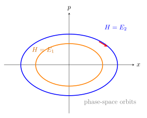
图 7:classical harmonic oscillator 的定能轨道是 phase-space ellipse;canonical ensemble 对各椭圆按 \(e^{-\beta E}\) 加权。
3.2 均方涨落直接连接温度
Gaussian distribution 给
\[\left\langle\frac{p^2}{2m}\right\rangle=\frac12k_BT, \qquad \left\langle\frac12k_sx^2\right\rangle=\frac12k_BT,\]
所以
\[\boxed{\langle x^2\rangle=\frac{k_BT}{k_s}}, \qquad \boxed{\langle p^2\rangle=mk_BT}.\]
均值 \(\langle x\rangle=\langle p\rangle=0\) 来自分布对称性,不意味着粒子静止。
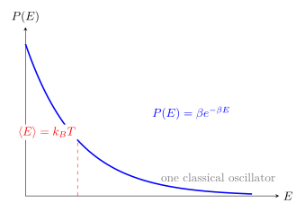
图 8:classical oscillator 的能量呈 exponential distribution,平均值为 \(k_BT\),并非每个振子都恰有该能量。
Worked Example 3 — 热平衡谐振子的均方振幅与动量
已知条件: 一维振子 \(m=1.00\times10^{-24}\ \mathrm{kg}\)、\(k_s=10.0\ \mathrm{N\,m^{-1}}\),\(T=300\ \mathrm K\)。求 \(U,C_V,x_{rms},p_{rms}\)。
研究对象: 单个一维 classical oscillator。
系统边界与坐标: 与热库接触;\(x=0\) 为势能最低点,正负方向任取但固定。
模型及理由: Hamiltonian 在 \(p,x\) 中都是二次型,且先假定 \(k_BT\gg\hbar\omega\) 使 classical continuum 近似成立。
\[k_BT=(1.380649\times10^{-23})(300) =4.141947\times10^{-21}\ \mathrm J.\]
\[U=k_BT=4.14195\times10^{-21}\ \mathrm J, \qquad C_V=k_B=1.380649\times10^{-23}\ \mathrm{J\,K^{-1}}.\]
\[x_{rms}=\sqrt{\frac{k_BT}{k_s}} =2.035\times10^{-11}\ \mathrm m,\]
\[p_{rms}=\sqrt{mk_BT} =6.436\times10^{-23}\ \mathrm{kg\,m\,s^{-1}}.\]
检查与解释: \(k_sx_{rms}^2\) 与 \(p_{rms}^2/m\) 都等于 \(k_BT\);\(\langle x\rangle=0\) 但 rms 非零。这里 \(\omega=\sqrt{k_s/m}=3.162\times10^{12}\ \mathrm{s^{-1}}\),故 \(\hbar\omega/(k_BT)=0.0805\ll1\),classical approximation 自洽;不能仅因温度数值“大”就跳过此检查。
Knowledge 4 — Equipartition and its breakdown / 能量均分及其失效
Knowledge ID: P03-U06-L03-K04
4.1 每个独立二次项贡献 \(k_BT/2\)
若某个连续变量 \(y\) 在 Hamiltonian 中以 \(ay^2\) 的独立二次项出现,积分边界使分部积分的边界项消失,则
\[\left\langle y\frac{\partial H}{\partial y}\right\rangle=k_BT.\]
对 \(H_y=ay^2\),\(y\,\partial H/\partial y=2H_y\),于是
\[\boxed{\langle H_y\rangle=\frac12k_BT}.\]
若每个粒子或分子含 \(f\) 个 active independent quadratic terms,则 \(N\) 粒子系统有
\[U=\frac f2Nk_BT, \qquad C_V=\frac f2Nk_B,\]
但 \(f\) 必须数单个粒子或分子的 Hamiltonian 中实际独立并热可访问的二次项,不能只数几何坐标。若改用全系统二次项总数 \(f_{\mathrm{tot}}\),则 \(U=(f_{\mathrm{tot}}/2)k_BT\),不再额外乘 \(N\)。
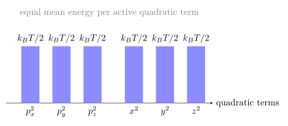
图 9:equipartition 是对独立二次能量项的平均分账,不是“每种粒子或每个坐标各得相同总能量”。
4.2 Quantum freeze-out 是经典均分最重要的边界
若一个 mode 的量子能级间隔 \(\Delta E\) 满足 \(k_BT\ll\Delta E\),激发概率指数受抑制,该 mode 不再贡献 classical \(k_B/2\) 或 \(k_B\)。典型判据:
\[\eta=\frac{\Delta E}{k_BT}.\]
\(\eta\ll1\) 时能级近似连续,classical equipartition 通常良好;\(\eta\gtrsim1\) 时出现 freeze-out。对 oscillator,精确 quantum heat capacity 为
\[C_{V,q}=k_B \left(\frac{\hbar\omega}{k_BT}\right)^2 \frac{e^{\hbar\omega/(k_BT)}}{\left(e^{\hbar\omega/(k_BT)}-1\right)^2},\]
它在高温趋于 \(k_B\)、低温趋于零。不可分辨量子粒子、旋转/振动离散能谱、强相互作用、约束或非二次项也会使简单计数失效。
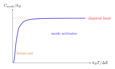
图 10:离散 mode 的热容由低温冻结区上升到高温 classical equipartition limit;曲线为定性示意。
Worked Example 4 — 双原子气体的 active-mode bookkeeping
已知条件: 一摩尔理想线性双原子气体。情形 A:三平动与两转动二次项已按 classical equipartition 激活,振动冻结;情形 B:一个振动 mode 的动能与势能二次项也完全激活。取 \(T=300.0\ \mathrm K\),比较 \(U,C_V,C_p,\gamma\)。
研究对象: 一摩尔气体;忽略电子激发与相互作用。
系统边界与参考系: 平衡、无宏观流动;\(U\) 不含整体质心运动。
模型及理由: 情形 A 有 \(f=5\),情形 B 有 \(f=7\);理想气体 \(C_p=C_V+R\)。
情形 A:
\[U_A=\frac52RT=6.23585\times10^3\ \mathrm J,\]
\[C_{V,A}=\frac52R=20.7862\ \mathrm{J\,mol^{-1}K^{-1}},\]
\[C_{p,A}=\frac72R=29.1006\ \mathrm{J\,mol^{-1}K^{-1}}, \qquad \gamma_A=\frac75=1.400.\]
情形 B:
\[U_B=\frac72RT=8.73019\times10^3\ \mathrm J,\]
\[C_{V,B}=\frac72R=29.1006\ \mathrm{J\,mol^{-1}K^{-1}}, \qquad C_{p,B}=\frac92R=37.4151\ \mathrm{J\,mol^{-1}K^{-1}},\]
\[\gamma_B=\frac97=1.286.\]
有效数字与检查: 每增加一个 fully active vibration,\(U\) 增加 \(RT\)、\(C_V\) 增加 \(R\),因为它含 kinetic 与 potential 两个二次项。
物理解释与边界: 不能据 \(T=300\ \mathrm K\) 自动决定真实分子的情形;必须把 \(k_BT\) 与该分子的 rotational/vibrational spacing 比较。情形 B 是高温极限模型,不声称所有双原子分子在 300 K 振动已完全激活。
Lesson synthesis / 全课整合
三个应用共享同一算法:从 Hamiltonian 识别自由度和约束,构造无量纲 \(Z\),再用对数导数获得宏观量。自由粒子的位置积分产生 \(V\)、动量 Gaussian 产生 \(T^{3/2}\),所以得到 ideal-gas pressure 和 \(3k_BT/2\);二态磁矩的 \(2\cosh x\) 产生 \(\tanh x\) 磁化和中温热容峰;谐振子的两个 Gaussian 各贡献 \(k_BT/2\)。Equipartition 是这些 Gaussian 结果的统一表达,但只有在连续 classical states 被充分热采样时成立。
建模流程: 写 Hamiltonian 与系统边界 → 判断粒子可分辨性及经典参数 → 分解可积自由度 → 构造 \(Z\) → 求 \(F,U\) 与 generalized response → 检查低温、高温、弱场、稀薄和饱和极限 → 若 \(\Delta E/(k_BT)\gtrsim1\),改用 quantum partition function。
Formula-and-decision table / 公式—决策表
| Model task | Relation | Use only when | Key caution |
|---|---|---|---|
| thermal wavelength | \(\lambda_T=h/\sqrt{2\pi mk_BT}\) | free-particle Gaussian momentum integral | convention tied to \(2\pi\) choice |
| classical ideal-gas \(Z_N\) | \(Z_N=(V/\lambda_T^3)^N/N!\) | dilute identical noninteracting particles | require \(n\lambda_T^3\ll1\) |
| ideal-gas thermodynamics | \(pV=Nk_BT\), \(U=3Nk_BT/2\) | monatomic point particles | internal modes absent |
| two-state magnet | \(Z=(2\cosh x)^N\) | independent fixed moments, \(x=\mu_mB/(k_BT)\) | ignore interactions and level complexity |
| magnetization | \(\mathcal M=N\mu_m\tanh x\) | same model | distinguish total moment from magnetization density |
| oscillator partition function | \(z_{ho}=k_BT/(\hbar\omega)\) | classical one-dimensional oscillator | fails when \(k_BT\lesssim\hbar\omega\) |
| equipartition | \(\langle H_y\rangle=k_BT/2\) | independent quadratic term with valid boundaries | count active terms, not labels |
| quantum freeze-out test | \(\eta=\Delta E/(k_BT)\) | discrete spectrum known | \(\eta\gtrsim1\) needs quantum treatment |
Model boundaries / 模型边界
- Ideal-gas factorization assumes negligible interactions; virial corrections enter when density or interaction range grows.
- \(N!\) corrects label overcounting in classical identical-particle thermodynamics but does not replace Bose or Fermi symmetrization when \(n\lambda_T^3\) is not small.
- Two-state paramagnet ignores dipole–dipole or exchange interactions; Curie law fails near magnetic ordering and saturation.
- The oscillator phase-space integral is classical and uses an arbitrary \(h\) cell; its absolute free energy must not be extrapolated below the quantum regime.
- Simple equipartition requires accessible continuous degrees of freedom and convergent boundary terms; constraints and bounded spectra require direct \(Z\) calculation.
- A mode can be mechanically present but thermally frozen; active degree count is temperature dependent when energy levels are discrete.
Misconception clinic / 易错概念诊所
- “经典 ideal-gas partition function 不应出现 \(h\)。” 错;连续相空间计数需无量纲 cell,虽然 \(pV\) 和 \(U\) 等经典结果中 \(h\) 消去。
- “除以 \(N!\) 就已经完整处理量子不可分辨性。” 错;它只给 dilute Maxwell–Boltzmann limit。
- “顺磁体总有 \(\mathcal M\propto B/T\)。” 错;Curie linear law 只在 \(\mu_mB\ll k_BT\),强场会饱和。
- “\(\langle x\rangle=0\) 表示谐振子不动。” 错;\(\langle x^2\rangle=k_BT/k_s\) 非零。
- “每个自由度贡献 \(k_BT/2\),所以振动只加 \(k_BT/2\)。” 错;一个 classical vibration 有动能与势能两个二次项,共加 \(k_BT\)。
- “低温热容偏离 equipartition 是能量不守恒。” 错;能量仍守恒,偏离来自离散能谱使部分 mode 无法被热激发。
Practice and retrieval / 练习与检索
1. Thermal wavelength scaling(K01)
温度增为四倍时 \(\lambda_T\) 如何变化?质量增为九倍时呢?
Answer
\(\lambda_T\propto(mT)^{-1/2}\)。温度乘 \(4\) 或质量乘 \(4\) 都使其减半;质量乘 \(9\) 使其变为原来的 \(1/3\)。
2. Classical-limit parameter(K01)
\(n=1.0\times10^{25}\ \mathrm{m^{-3}}\)、\(\lambda_T=2.0\times10^{-9}\ \mathrm m\)。计算 \(n\lambda_T^3\) 并判断 classical dilute formula。
Answer
\(n\lambda_T^3=(1.0\times10^{25})(2.0\times10^{-9})^3=0.080\)。它小于 \(1\) 但未极小;classical approximation 可能尚可作首近似,精密计算应评估 quantum-statistical correction。
3. Ideal-gas derivative(K01)
由 \(\ln Z_N=N\ln V+\text{terms independent of }V\) 推出压强。
Answer
\(p=k_BT(\partial\ln Z_N/\partial V)_{T,N}=k_BTN/V\),故 \(pV=Nk_BT\)。
4. Curie limit(K02)
从 \(\tanh x\approx x\) 推出弱场磁化,并写出适用条件。
Answer
\(\mathcal M=N\mu_m\tanh x\approx N\mu_m^2B/(k_BT)\);要求 \(x=\mu_mB/(k_BT)\ll1\) 且磁矩间相互作用可忽略。
5. 磁化饱和(K02)
固定 \(B>0\),\(T\to0\) 时 \(\mathcal M,U,C_B\) 各趋向什么?
Answer
\(x\to\infty\),所以 \(\mathcal M\to N\mu_m\)、\(U\to-N\mu_mB\)、\(C_B\to0\)。系统几乎全处于顺场基态。
6. Oscillator Gaussian(K03)
若 \(k_s\) 增为四倍、\(T\) 不变,\(x_{rms}\) 如何变化?
Answer
\(x_{rms}=\sqrt{k_BT/k_s}\),因此变为原来的一半;平均势能仍为 \(k_BT/2\)。
7. 三维谐振子(K03, K04)
一个三维 isotropic classical oscillator 的 \(U\) 与 \(C_V\) 是多少?
Answer
三个动量平方项加三个坐标平方项,共 \(f=6\),所以 \(U=3k_BT\)、\(C_V=3k_B\) 每振子。
8. 双原子自由度(K04)
线性双原子气体若平动和转动激活、振动冻结,molar \(C_V\) 是多少?
Answer
平动三项、转动两项,共 \(f=5\),所以 \(C_{V,m}=5R/2=20.8\ \mathrm{J\,mol^{-1}K^{-1}}\)。
9. Freeze-out criterion(K04)
某 mode 的 \(\Delta E=0.100\ \mathrm{eV}\),\(T=300\ \mathrm K\)。估算 \(\eta=\Delta E/(k_BT)\) 并判断。
Answer
\(k_BT\approx0.02585\ \mathrm{eV}\),所以 \(\eta\approx3.87\)。激发明显受抑制,不能给它完整 classical equipartition contribution。
10. 综合模型审计(K01–K04)
实验气体热容低于 classical active-mode prediction。给出三项在改公式前必须检查的物理原因。
Answer
检查 rotational/vibrational quantum freeze-out、气体是否单原子或分子结构不同、相互作用与非理想性、量子简并参数 \(n\lambda_T^3\)、化学反应或 dissociation,以及是否比较了 \(C_p\) 与 \(C_V\) 的不同实验条件。
Exit ticket / 课末检验
- 从 free-particle Hamiltonian 写出 \(Z_N\),并在每个因子旁说明 \(V\)、\(T^{3N/2}\)、\(h^{3N}\) 与 \(N!\) 分别从何而来。
- 任选 paramagnet 或 oscillator,用“精确 \(Z\) → 高温极限 → 低温失效”三步说明 equipartition 是近似结论而非无条件定律。
References and source notes / 参考资料与来源说明
- MIT OCW RES.8-010, Lecture 7 — Statistical Physics of the Ideal Gas — classical ideal-gas partition function、thermal wavelength、\(N!\) and equation of state。
- MIT OCW 8.333, Lecture 13 — Ideal Gas and Canonical Ensemble — phase-space measure、ideal gas、canonical derivation and Gibbs paradox boundary。
- UC San Diego 8.044 Notes, Chapter 6 — Statistical Mechanics at Fixed Temperature — ideal gas、two-level systems、classical oscillators、equipartition and paramagnetism。
- University of Colorado Boulder PHYS 4230 — Statistical Mechanics and Thermodynamics — canonical lecture set cross-checking paramagnet、oscillator、equipartition and Boltzmann ideal gas。
- University of Texas at Austin — Thermodynamics and Statistical Mechanics — official university notes on partition functions、paramagnetism、equipartition and harmonic oscillators。
- MIT OCW 3.012, Lecture 23/24 Materials on Boltzmann Factor and Oscillators — Boltzmann factor、partition function and oscillator heat-capacity transition to quantum treatment。
- NIST Fundamental Constants in Nature — exact SI \(k_B\)、\(N_A\) and relation \(R=N_Ak_B\) used in examples。
以上链接均于 2026-08-25 实际打开并核对到具体 PDF、大学课程页或 NIST 官方页面。正文采用统一 SI 记号,数值使用 exact SI constants 复算;所有 phase-space、函数与能量图均为按本文方程原创的教学示意。
Source-to-content map
| Source | Used for | Knowledge ID / Section | Model boundary or convention |
|---|---|---|---|
| MIT RES.8-010 Lecture 7 | ideal-gas \(Z_N\), \(N!\), thermodynamics | K01 | dilute Maxwell–Boltzmann regime |
| MIT 8.333 Lecture 13 | phase-space counting and canonical gas | K01 | identical-particle correction retained |
| UCSD 8.044 Chapter 6 | paramagnet, oscillator, equipartition | K02, K03, K04 | fixed-moment and classical-mode assumptions |
| Colorado PHYS 4230 | independent cross-check of applications | K01–K04 | lecture notation translated to this contract |
| UT Austin notes | equipartition theorem and breakdown examples | K02–K04 | direct \(Z\) preferred outside quadratic limit |
| MIT 3.012 notes | oscillator partition function and quantum heat capacity | K03, K04 | quantum energy spacing marks boundary |
| NIST constants | numerical values of \(k_B,N_A,R\) | examples | exact SI constants |
复习与拓展
- Unit 3.7 将在 \(n\lambda_T^3\gtrsim1\) 时以 Bose–Einstein 与 Fermi–Dirac statistics 替代 Maxwell–Boltzmann counting。
- Solid-state physics 会把 independent oscillator 模型扩展为 phonon spectrum,导出 Einstein 与 Debye heat capacities。
- Magnetism 课程会加入 exchange interaction、collective order 和 Ising model,解释 Curie law 的失效与相变。
- Unit 3.8 将把 Maxwell distribution 与碰撞结合,导出 diffusion、viscosity and thermal transport。