
Learning objectives / 学习目标
完成本课后,你应当能够:
- 按统一方向约定定义两点电荷及一般电荷分布的电偶极矩,并判断它对坐标原点的依赖。
- 推导永久电偶极子在匀强场中的合力、力矩与势能,区分稳定和不稳定平衡。
- 推导短偶极子在非匀强静电场中的首阶合力,并区分永久偶极与感生偶极的能量公式。
- 写出有限两点电荷偶极子在轴线和中垂面上的精确场,并量化远场近似的误差。
- 从精确 Coulomb 势的 Taylor 展开得到点偶极势与场,解释其角分布和 \(r^{-3}\) 场强衰减。
- 将局域电荷分布的势展开到 monopole、dipole、quadrupole 阶,并在明确的四极矩 convention 下计算例子。
- 根据总电荷、反演对称性和最低非零多极矩判断远场主导阶,同时说明模型边界。
0. Before starting: notation, units, and the forward use of potential
0.1 Source point and field point must remain distinct
本课始终使用:
| Symbol | Meaning | Unit |
|---|---|---|
| \(\mathbf r'\) | source coordinate / 源点坐标 | m |
| \(\mathbf r\) | field-point coordinate / 场点坐标 | m |
| \(\mathbf R=\mathbf r-\mathbf r'\) | source-to-field displacement | m |
| \(\rho(\mathbf r')\) | volume charge density at the source | \(\mathrm{C\,m^{-3}}\) |
| \(k_e\) | \(1/(4\pi\varepsilon_0)\) | \(\mathrm{N\,m^2\,C^{-2}}\) |
\[\boxed{k_e\equiv\frac{1}{4\pi\varepsilon_0}} \approx8.987\,551\,786\times10^9\ \mathrm{N\,m^2\,C^{-2}}.\]
0.2 Electric potential is used here as a forward tool
严格的课程顺序将在 Unit 4.3 系统学习电势。本课为高效处理远场,先局部使用三条关系:
\[\phi(\mathbf r) =k_e\int\frac{\rho(\mathbf r')}{|\mathbf r-\mathbf r'|}\,d^3r', \qquad \mathbf E=-\boldsymbol\nabla\phi, \qquad U=q\phi.\]
它们在本课中是前瞻工具(forward preview),并不替代 Unit 4.3 对电势、路径无关性和 Poisson 方程的完整讨论。
0.3 Three distinct objects
| Object | Definition | Physical role |
|---|---|---|
| finite dipole | two finite charges \(\pm q\) separated by \(\mathbf d\) | exact two-charge model |
| point or ideal dipole | \(d\to0\) while \(p=qd\) is held fixed | leading far-field source model |
| general dipole moment | \(\mathbf p=\int\rho\mathbf r'\,d^3r'\) | first moment of any localized distribution |
Knowledge 1 — Electric dipole moment / 电偶极矩
1.1 Definition and direction convention
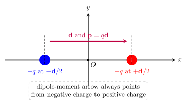
令 \(-q\) 位于 \(-\mathbf d/2\),\(+q\) 位于 \(+\mathbf d/2\)。分离矢量 \(\mathbf d\) 从负电荷指向正电荷,定义
\[\boxed{\mathbf p\equiv q\mathbf d}.\]
- 方向:\(-q\rightarrow+q\);
- 大小:\(p=qd\);
- SI 单位:\(\mathrm{C\,m}\);
- \(\mathbf p\) 是电荷分布的一阶矩,不是力,也不是线动量。
1.2 General localized charge distribution
对离散点电荷:
\[\boxed{\mathbf p=\sum_a q_a\mathbf r'_a}.\]
对连续分布:
\[\boxed{\mathbf p=\int\rho(\mathbf r')\,\mathbf r'\,d^3r'}.\]
若电荷只分布在线或面上,分别把 \(\rho\,d^3r'\) 换成 \(\lambda\,d\ell'\) 或 \(\sigma\,dA'\)。
对于两点电荷,以中点为原点:
\[\mathbf p =(+q)\frac{\mathbf d}{2} +(-q)\left(-\frac{\mathbf d}{2}\right) =q\mathbf d.\]
分子的偶极矩常用 debye(D)表示:
\[1\ \mathrm D=3.335\,64\times10^{-30}\ \mathrm{C\,m}.\]
这里的 debye 是偶极矩单位,与 plasma physics 中的 Debye length 没有概念关系。
1.3 Origin dependence
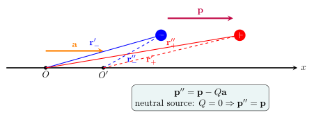
若把原点平移 \(\mathbf a\),同一源点的新坐标为
\[\mathbf r''=\mathbf r'-\mathbf a.\]
于是
\[\mathbf p'' =\int\rho(\mathbf r')(\mathbf r'-\mathbf a)\,d^3r' =\mathbf p-Q\mathbf a,\]
其中
\[Q\equiv\int\rho(\mathbf r')\,d^3r'.\]
因此
\[\boxed{Q=0\quad\Longrightarrow\quad\mathbf p\ \text{is origin independent}.}\]
若 \(Q\ne0\),偶极矩会随原点变化;此时远场首项本来就是 monopole,不能把某个任意原点下的 \(\mathbf p\) 当作独立于坐标的绝对属性。12
1.4 Symmetry can force \(\mathbf p=0\)
若相对于原点
\[\rho(-\mathbf r')=\rho(\mathbf r'),\]
则 \(\rho(\mathbf r')\mathbf r'\) 是奇函数,积分为零:\(\mathbf p=0\)。例如具有反演中心的电荷分布没有永久电偶极矩。
反之,\(Q=0\) 并不自动保证 \(\mathbf p\ne0\):中性只消去 monopole;是否存在 dipole 还由正、负电荷的空间分离与对称性决定。
1.5 Worked Example 1 — A finite SI dipole
两电荷 \(\pm3.0\ \mathrm{nC}\) 相距 \(4.0\ \mathrm{mm}\),从负电荷指向正电荷的方向为 \(+x\):
\[p=qd =(3.0\times10^{-9})(4.0\times10^{-3}) =\boxed{1.20\times10^{-11}\ \mathrm{C\,m}}.\]
\[\boxed{\mathbf p=(1.20\times10^{-11}\ \mathrm{C\,m})\,\hat{\mathbf x}}.\]
若整体把两电荷同时平移,\(Q=+q-q=0\),所以关于任何原点计算都得到同一 \(\mathbf p\)。
Knowledge 2 — Torque and energy of a dipole in a field / 偶极子在电场中的力矩与能量
2.1 Uniform field: zero net force but generally nonzero torque
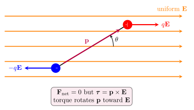
把有限偶极子置于匀强外电场 \(\mathbf E\),两端受力
\[\mathbf F_+=q\mathbf E, \qquad \mathbf F_-=-q\mathbf E.\]
因此
\[\boxed{\mathbf F_{\rm net}=\mathbf F_++\mathbf F_-=0}.\]
关于偶极中点的合力矩是
\[\boldsymbol\tau =\frac{\mathbf d}{2}\times q\mathbf E +\left(-\frac{\mathbf d}{2}\right)\times(-q\mathbf E) =q\mathbf d\times\mathbf E,\]
即
\[\boxed{\boldsymbol\tau=\mathbf p\times\mathbf E}, \qquad \boxed{\tau=pE\sin\theta}.\]
其中 \(\theta\) 是 \(\mathbf p\) 与 \(\mathbf E\) 的夹角;叉积方向决定真实转动轴。34
2.2 Orientation energy
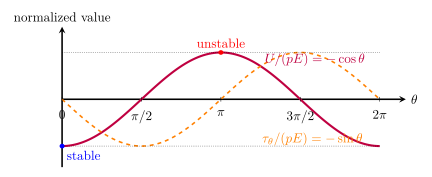
取 \(\theta=\pi/2\) 为零势能参考。外力缓慢转动偶极子时,
\[dU=-\tau_{\rm field}\,d\theta,\]
积分得到
\[\boxed{U(\theta)=-pE\cos\theta=-\mathbf p\cdot\mathbf E}.\]
| Orientation | Energy | Equilibrium |
|---|---|---|
| \(\mathbf p\parallel\mathbf E\),\(\theta=0\) | \(U=-pE\) | stable / 稳定 |
| \(\mathbf p\perp\mathbf E\),\(\theta=\pi/2\) | \(U=0\) | not equilibrium unless constrained |
| \(\mathbf p\parallel(-\mathbf E)\),\(\theta=\pi\) | \(U=+pE\) | unstable / 不稳定 |
若规定正 \(\theta\) 方向为逆时针,场的广义力矩分量满足
\[\boxed{\tau_\theta=-\frac{dU}{d\theta}=-pE\sin\theta}.\]
“力矩大小 \(pE\sin\theta\)”与“有符号恢复力矩 \(-pE\sin\theta\)”必须区分。
2.3 Nonuniform field: leading force on a short permanent dipole
设偶极中心在 \(\mathbf r\)。精确合力为
\[\mathbf F_{\rm exact} =q\mathbf E\!\left(\mathbf r+\frac{\mathbf d}{2}\right) -q\mathbf E\!\left(\mathbf r-\frac{\mathbf d}{2}\right).\]
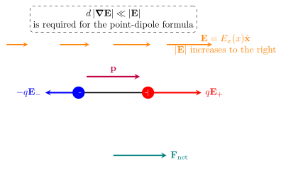
若外场在距离 \(d\) 上缓慢变化,Taylor 展开:
\[\mathbf E\!\left(\mathbf r\pm\frac{\mathbf d}{2}\right) =\mathbf E(\mathbf r) \pm\frac12(\mathbf d\cdot\boldsymbol\nabla)\mathbf E +O(d^2).\]
相减后偶数阶消去,得到
\[\boxed{\mathbf F=(\mathbf p\cdot\boldsymbol\nabla)\mathbf E}\]
以及首阶力矩
\[\boxed{\boldsymbol\tau\simeq\mathbf p\times\mathbf E(\mathbf r)}.\]
若 \(\mathbf p\) 在空间中视为常量,向量恒等式给出
\[\boldsymbol\nabla(\mathbf p\cdot\mathbf E) =(\mathbf p\cdot\boldsymbol\nabla)\mathbf E +\mathbf p\times(\boldsymbol\nabla\times\mathbf E).\]
在静电场中 \(\boldsymbol\nabla\times\mathbf E=0\),所以
\[\boxed{\mathbf F=(\mathbf p\cdot\boldsymbol\nabla)\mathbf E =\boldsymbol\nabla(\mathbf p\cdot\mathbf E) =-\boldsymbol\nabla U}.\]
离开静电、固定 \(\mathbf p\) 的条件后,这两种写法不能不加说明地互换。25
2.4 Permanent versus induced dipoles
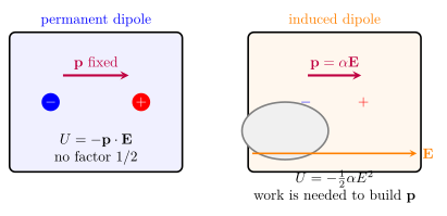
对给定的永久偶极矩,能量是
\[U_{\rm perm}=-\mathbf p\cdot\mathbf E.\]
对各向同性、线性、可极化的小物体,若
\[\mathbf p_{\rm ind}=\alpha\mathbf E,\]
建立偶极矩本身也需要逐步极化;正确能量为
\[\boxed{U_{\rm ind}=-\frac12\alpha E^2}\]
而不是把 \(\mathbf p=\alpha\mathbf E\) 直接代入永久偶极公式。于是
\[\boxed{\mathbf F_{\rm ind}=\frac12\alpha\boldsymbol\nabla(E^2)}\]
(静电、标量且位置无关的 \(\alpha>0\))。这里的 \(\mathbf E\) 是不含粒子自场的外部驱动场,并假定固定外部场源、无永久偶极、极化可逆且处在线性响应区;一般非线性响应应使用 \(U_{\rm ind}=-\int_{\mathbf 0}^{\mathbf E}\mathbf p_{\rm ind}(\mathbf E')\cdot d\mathbf E'\),不能机械保留 \(1/2\)。各向同性感生偶极与局域场平行,因而没有 \(\mathbf p\times\mathbf E\) 力矩;各向异性极化率则可能产生取向力矩。6
2.5 Worked Example 2 — Torque and energy in a uniform field
沿用 \(p=1.20\times10^{-11}\ \mathrm{C\,m}\),置于
\[E=2.50\times10^4\ \mathrm{N\,C^{-1}}, \qquad \theta=30.0^\circ.\]
力矩大小:
\[\tau=pE\sin\theta =(1.20\times10^{-11})(2.50\times10^4)\sin30^\circ =\boxed{1.50\times10^{-7}\ \mathrm{N\,m}}.\]
以 \(U=0\) at \(90^\circ\):
\[U=-pE\cos\theta =\boxed{-2.60\times10^{-7}\ \mathrm J}.\]
合力仍严格为零,因为外场均匀。
2.6 Worked Example 3 — Force in a one-dimensional gradient
刚性永久偶极沿 \(+x\),
\[p_x=6.0\times10^{-12}\ \mathrm{C\,m},\]
外场在偶极附近为
\[\mathbf E(x)=(E_0+Gx)\hat{\mathbf x}, \qquad G=3.0\times10^6\ \mathrm{V\,m^{-2}}.\]
则
\[F_x=p_x\frac{\partial E_x}{\partial x} =p_xG =\boxed{1.8\times10^{-5}\ \mathrm N}.\]
方向为 \(+x\)。若把同一永久偶极反向固定,\(p_x<0\),力也反向;这再次说明永久偶极并非无条件朝 \(|E|\) 较大处运动。
2.7 Model boundary
Knowledge 3 — Dipole field and far-field approximation / 偶极场与远场近似
3.1 Exact potential and field of two finite charges
继续令 \(+q\) 位于 \(+\mathbf d/2\),\(-q\) 位于 \(-\mathbf d/2\)。对任意场点 \(\mathbf r\),精确势为
\[\boxed{ \phi_{\rm exact}(\mathbf r) =k_eq\left[ \frac{1}{|\mathbf r-\mathbf d/2|} -\frac{1}{|\mathbf r+\mathbf d/2|} \right] }.\]
直接叠加两点电荷场:
\[\boxed{ \mathbf E_{\rm exact}(\mathbf r) =k_eq\left[ \frac{\mathbf r-\mathbf d/2}{|\mathbf r-\mathbf d/2|^3} -\frac{\mathbf r+\mathbf d/2}{|\mathbf r+\mathbf d/2|^3} \right] }.\]
这两式对源点之外的任意位置成立,没有使用 \(r\gg d\)。远场公式必须从它们近似得到,不能反过来拿远场公式计算靠近某一个电荷的场。
3.2 Exact special cases: axis and equatorial plane
令 \(\mathbf p=p\hat{\mathbf z}\),两电荷位于 \(z=\pm a\),其中
\[a=\frac d2, \qquad p=2qa.\]
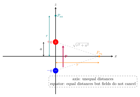
On the positive axis / 正轴线,\(r>a\)
电势:
\[\phi_{\rm ax}^{\rm exact}(r) =k_eq\left(\frac1{r-a}-\frac1{r+a}\right) =\boxed{\frac{k_ep}{r^2-a^2}}.\]
电场沿 \(+\hat{\mathbf z}=\hat{\mathbf p}\):
\[\boxed{ \mathbf E_{\rm ax}^{\rm exact}(r) =\frac{2k_epr}{(r^2-a^2)^2}\,\hat{\mathbf p} }.\]
在负轴线一侧,电势变号,但场仍沿 \(\hat{\mathbf p}\);上式的场强大小可用 \(r\) 表示从中心到场点的正距离。
On the equatorial plane / 中垂面
两电荷到场点距离相等,所以电势精确为零:
\[\boxed{\phi_{\rm eq}^{\rm exact}=0}.\]
但两场的横向分量抵消、沿偶极轴的分量同向相加:
\[\boxed{ \mathbf E_{\rm eq}^{\rm exact}(r) =-\frac{k_ep}{(r^2+a^2)^{3/2}}\,\hat{\mathbf p} }.\]
3.3 Far-field derivation from the exact potential
若
\[r\gg d,\]
则对 \(|\mathbf r'|<r\),Coulomb kernel 的前几项为
\[\frac1{|\mathbf r-\mathbf r'|} =\frac1r +\frac{\hat{\mathbf r}\cdot\mathbf r'}{r^2} +O\!\left(\frac{r'^2}{r^3}\right).\]
分别令 \(\mathbf r'=\pm\mathbf d/2\):
\[\frac1{|\mathbf r-\mathbf d/2|} \simeq\frac1r+\frac{\hat{\mathbf r}\cdot\mathbf d}{2r^2},\]
\[\frac1{|\mathbf r+\mathbf d/2|} \simeq\frac1r-\frac{\hat{\mathbf r}\cdot\mathbf d}{2r^2}.\]
相减时两个 \(1/r\) monopole 项抵消:
\[\phi_{\rm dip}(\mathbf r) =k_eq\frac{\hat{\mathbf r}\cdot\mathbf d}{r^2} =\boxed{k_e\frac{\mathbf p\cdot\hat{\mathbf r}}{r^2}}.\]
等价地,
\[\boxed{ \phi_{\rm dip}(\mathbf r) =k_e\frac{\mathbf p\cdot\mathbf r}{r^3} =-k_e\mathbf p\cdot\boldsymbol\nabla\left(\frac1r\right) }.\]
对关于中点反对称的理想两电荷偶极,所有偶数 \(\ell\) 项消失,所以下一个修正是 octupole;相对误差从 \(O[(d/r)^2]\) 开始,而不是 \(O(d/r)\)。78
3.4 Point-dipole electric field
对 \(\mathbf p\) 为空间常矢量且 \(r\ne0\),
\[\mathbf E_{\rm dip} =-\boldsymbol\nabla\phi_{\rm dip} =-k_e\boldsymbol\nabla\left(\frac{\mathbf p\cdot\mathbf r}{r^3}\right).\]
利用
\[\boldsymbol\nabla(\mathbf p\cdot\mathbf r)=\mathbf p, \qquad \boldsymbol\nabla(r^{-3})=-3r^{-4}\hat{\mathbf r},\]
得到
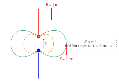
\[\boxed{ \mathbf E_{\rm dip}(\mathbf r) =\frac{k_e}{r^3} \left[3(\mathbf p\cdot\hat{\mathbf r})\hat{\mathbf r}-\mathbf p\right] }, \qquad r\ne0.\]
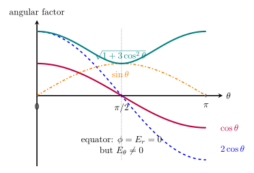
若 \(\mathbf p=p\hat{\mathbf z}\),球坐标分量为
\[\boxed{E_r=\frac{2k_ep\cos\theta}{r^3}}, \qquad \boxed{E_\theta=\frac{k_ep\sin\theta}{r^3}}, \qquad E_\varphi=0.\]
场强大小:
\[\boxed{ E(r,\theta) =\frac{k_ep}{r^3}\sqrt{1+3\cos^2\theta} }.\]
两条经典方向结果:
\[\boxed{\mathbf E_{\rm ax}\simeq\frac{2k_ep}{r^3}\hat{\mathbf p}}, \qquad \boxed{\mathbf E_{\rm eq}\simeq-\frac{k_ep}{r^3}\hat{\mathbf p}}.\]
轴线场强是同距离中垂面场强的两倍;两者方向相反。
3.5 Angular structure
在固定 \(r\) 上:
\[\frac{\phi}{k_ep/r^2}=\cos\theta, \quad \frac{E_r}{k_ep/r^3}=2\cos\theta, \quad \frac{E_\theta}{k_ep/r^3}=\sin\theta,\]
\[\frac{|\mathbf E|}{k_ep/r^3}=\sqrt{1+3\cos^2\theta}.\]
3.6 How far is “far”?
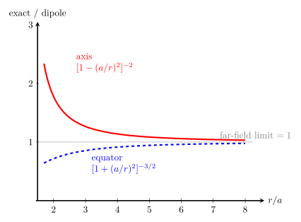
将精确轴线与中垂面场除以各自的点偶极远场:
\[\boxed{ \frac{E_{\rm ax}^{\rm exact}}{E_{\rm ax}^{\rm dip}} =\frac{1}{[1-(a/r)^2]^2} },\]
\[\boxed{ \frac{E_{\rm eq}^{\rm exact}}{E_{\rm eq}^{\rm dip}} =\frac{1}{[1+(a/r)^2]^{3/2}} }.\]
二者都在 \(r/a\to\infty\) 时趋近 1,但轴线近似从下方低估精确值,中垂面近似从上方高估精确值。
3.7 Worked Example 4 — Exact versus far-field numbers
取
\[q=2.0\ \mathrm{nC}, \qquad d=6.0\ \mathrm{mm}, \qquad a=3.0\ \mathrm{mm},\]
所以
\[p=qd=1.20\times10^{-11}\ \mathrm{C\,m}.\]
观察距离 \(r=4.0\ \mathrm{cm}\),即 \(r/a=13.3\)。
Positive axis
\[E_{\rm ax}^{\rm exact} =\frac{2k_epr}{(r^2-a^2)^2} =\boxed{3.409\times10^3\ \mathrm{N\,C^{-1}}},\]
\[E_{\rm ax}^{\rm dip} =\frac{2k_ep}{r^3} =\boxed{3.370\times10^3\ \mathrm{N\,C^{-1}}}.\]
远场值比精确值低 \(1.12\%\)。
Equatorial plane
\[E_{\rm eq}^{\rm exact} =\frac{k_ep}{(r^2+a^2)^{3/2}} =\boxed{1.671\times10^3\ \mathrm{N\,C^{-1}}},\]
\[E_{\rm eq}^{\rm dip} =\frac{k_ep}{r^3} =\boxed{1.685\times10^3\ \mathrm{N\,C^{-1}}}.\]
远场值比精确值高 \(0.845\%\)。方向为 \(-\hat{\mathbf p}\)。
3.8 Model boundary
Knowledge 4 — Multipole expansion and leading-order behavior / 多极展开与主导阶行为
4.1 The geometry and the small parameter
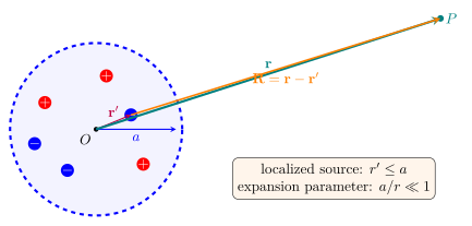
设所有源电荷位于以原点为中心、半径不超过 \(a\) 的有限区域:
\[|\mathbf r'|\le a.\]
观察点在源区之外,并满足
\[\boxed{r>a}, \qquad \text{far field: }\boxed{a/r\ll1}.\]
多极展开就是把 kernel \(1/|\mathbf r-\mathbf r'|\) 按无量纲小参数 \(r'/r\) 展开。9
4.2 Expanding the Coulomb kernel through quadrupole order
对 \(0\le r'<r\),Legendre 形式是
\[\frac1{|\mathbf r-\mathbf r'|} =\frac1r\sum_{\ell=0}^\infty \left(\frac{r'}r\right)^\ell P_\ell(\cos\gamma),\]
其中 \(\gamma\) 是 \(\mathbf r\) 与 \(\mathbf r'\) 的夹角。取前三阶:
\[\boxed{ \frac1{|\mathbf r-\mathbf r'|} =\frac1r +\frac{\hat{\mathbf r}\cdot\mathbf r'}{r^2} +\frac{3(\hat{\mathbf r}\cdot\mathbf r')^2-r'^2}{2r^3} +O\!\left(\frac{a^3}{r^4}\right) }.\]
代入
\[\phi(\mathbf r) =k_e\int\frac{\rho(\mathbf r')}{|\mathbf r-\mathbf r'|}\,d^3r'\]
并逐项定义:
\[\boxed{Q\equiv\int\rho(\mathbf r')\,d^3r'},\]
\[\boxed{p_i\equiv\int\rho(\mathbf r')x'_i\,d^3r'},\]
\[\boxed{ Q_{ij} \equiv \int\rho(\mathbf r') \left(3x'_ix'_j-r'^2\delta_{ij}\right)d^3r' }.\]
本课的势展开固定为
\[\boxed{ \phi(\mathbf r) =k_e\left[ \frac Qr +\frac{\mathbf p\cdot\hat{\mathbf r}}{r^2} +\frac{1}{2r^3}Q_{ij}\hat r_i\hat r_j +O(r^{-4}) \right] }.\]
这里及下文对重复 Cartesian indices 使用求和约定。该式与 MIT 8.07 公式表、Cambridge Part IB 讲义及常见 Jackson convention 一致。21011
4.3 Properties of the quadrupole tensor
由定义立即可得
\[Q_{ij}=Q_{ji}\]
和
\[Q_{ii} =\int\rho(3r'^2-3r'^2)\,d^3r'=0.\]
所以 \(Q_{ij}\) 是 symmetric and traceless:
\[\boxed{Q_{ij}=Q_{ji},\qquad\mathrm{Tr}\,Q=0}.\]
三维对称张量有 6 个独立分量,零迹去掉 1 个,因此电四极矩有 5 个独立分量,正好对应球谐展开中 \(\ell=2\) 的 \(m=-2,-1,0,1,2\)。
四极电场可从 \(\mathbf E_Q=-\nabla\phi_Q\) 得到。对 \(r\ne0\):
\[\boxed{ (E_Q)_i =\frac{k_e}{2r^4} \left[ 5(Q_{jk}\hat r_j\hat r_k)\hat r_i -2Q_{ij}\hat r_j \right] }.\]
它明确显示 quadrupole field 按 \(r^{-4}\) 衰减。
4.4 Leading-order behavior
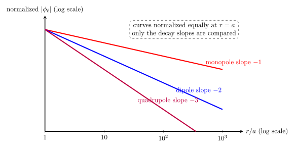
对一般 \(\ell\) 阶:
\[\boxed{\phi_\ell\propto r^{-(\ell+1)}}, \qquad \boxed{E_\ell\propto r^{-(\ell+2)}}.\]
| Lowest nonzero moment | Potential | Field | Angular character |
|---|---|---|---|
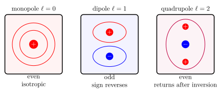
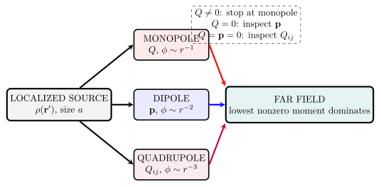
| monopole \(Q\),\(\ell=0\) | \(r^{-1}\) | \(r^{-2}\) | isotropic |
| dipole \(\mathbf p\),\(\ell=1\) | \(r^{-2}\) | \(r^{-3}\) | one positive and one negative potential lobe |
| quadrupole \(Q_{ij}\),\(\ell=2\) | \(r^{-3}\) | \(r^{-4}\) | two-sign, four-lobe or axial \(P_2\) pattern |
4.5 Symmetry and parity select the leading term
Legendre polynomial满足
\[P_\ell(-x)=(-1)^\ell P_\ell(x).\]
因此 \(\ell\) 阶势在空间反演下具有 parity \((-1)^\ell\):
\[\phi_\ell(-\mathbf r)=(-1)^\ell\phi_\ell(\mathbf r).\]
- even source symmetry \(\rho(-\mathbf r')=\rho(\mathbf r')\) 消去所有 odd moments,特别是 dipole;
- odd charge symmetry \(\rho(-\mathbf r')=-\rho(\mathbf r')\) 消去所有 even moments,包括 monopole 与 quadrupole;
- 轴对称会使许多 off-diagonal \(Q_{ij}\) 和 \(m\ne0\) spherical components 消失。
4.6 Canonical axial quadrupole
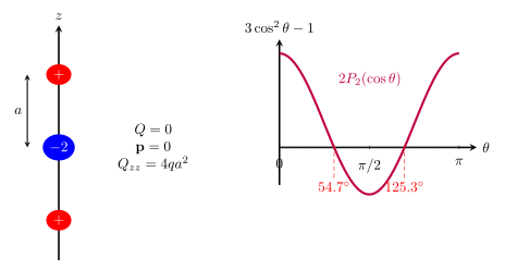
考虑
- \(+q\) at \(z=+a\);
- \(+q\) at \(z=-a\);
- \(-2q\) at the origin。
它满足
\[Q_{\rm total}=0, \qquad \mathbf p=0.\]
用本课 convention 逐点求和:
\[\boxed{ Q_{ij}=qa^2 \begin{pmatrix} -2&0&0\\ 0&-2&0\\ 0&0&4 \end{pmatrix} }.\]
代入 \(\hat r_x^2+\hat r_y^2=\sin^2\theta\)、\(\hat r_z^2=\cos^2\theta\):
\[\phi_Q(r,\theta) =\frac{k_eqa^2}{r^3}(3\cos^2\theta-1) =\boxed{\frac{2k_eqa^2}{r^3}P_2(\cos\theta)}.\]
零势锥面满足
\[3\cos^2\theta-1=0,\]
即
\[\boxed{\theta=54.74^\circ\quad\text{or}\quad125.26^\circ}.\]
4.7 Worked Example 5 — SI quadrupole potential
取
\[q=1.00\ \mathrm{nC}, \qquad a=2.00\ \mathrm{mm}, \qquad r=0.100\ \mathrm m.\]
张量分量:
\[Q_{zz}=4qa^2 =4(1.00\times10^{-9})(2.00\times10^{-3})^2 =\boxed{1.60\times10^{-14}\ \mathrm{C\,m^2}},\]
\[Q_{xx}=Q_{yy}=-2qa^2 =\boxed{-8.00\times10^{-15}\ \mathrm{C\,m^2}}.\]
正轴线 \(\theta=0\):
\[\phi_Q(r,0) =\frac{2k_eqa^2}{r^3} =\boxed{7.19\times10^{-2}\ \mathrm V}.\]
中垂面 \(\theta=\pi/2\):
\[\phi_Q\left(r,\frac\pi2\right) =-\frac{k_eqa^2}{r^3} =\boxed{-3.60\times10^{-2}\ \mathrm V}.\]
轴线首阶四极场为
\[E_r(r,0) =-\frac{\partial}{\partial r} \left(\frac{2k_eqa^2}{r^3}\right) =\frac{6k_eqa^2}{r^4} =\boxed{2.16\ \mathrm{N\,C^{-1}}}.\]
这里 \(r/a=50\),忽略更高阶是良好近似。
4.8 Origin dependence beyond the dipole
在原点平移 \(\mathbf a\)、新坐标 \(\mathbf r''=\mathbf r'-\mathbf a\) 下:
\[Q''=Q,\]
\[\mathbf p''=\mathbf p-Q\mathbf a,\]
而本课的 traceless quadrupole tensor 变为
\[\boxed{ Q''_{ij} =Q_{ij} -3(a_ip_j+a_jp_i) +2\delta_{ij}(\mathbf a\cdot\mathbf p) +Q(3a_ia_j-a^2\delta_{ij}) }.\]
因此:
- \(Q\) 对原点总是不变;
- \(\mathbf p\) 仅在 \(Q=0\) 时对原点不变;
- 若 \(Q=0\) 且 \(\mathbf p=0\),则 \(Q_{ij}\) 对任意原点平移保持不变;否则一般会随平移改变。
完整电势当然不依赖我们选哪一个原点;变化的是截断展开中各阶之间如何重新分配。通常把原点选在源区的几何中心、对称中心或能尽量消去低阶矩的位置。1
4.9 UG2 extension — Multipoles in an external potential
Energy expansion in a slowly varying external field
对一个小型电荷分布,外部势在原点附近缓慢变化: \[U_{\rm ext}=\int\rho(\mathbf r')\phi_{\rm ext}(\mathbf r')\,d^3r'.\] Taylor 展开并假定展开点附近无外部电荷,因此 \(\nabla^2\phi_{\rm ext}=0\),在本课 quadrupole convention 下: \[\boxed{ U_{\rm ext} =Q\phi_{\rm ext}(0) -\mathbf p\cdot\mathbf E_{\rm ext}(0) -\frac16Q_{ij}\,\partial_iE_{{\rm ext},j}(0) +\cdots }.\] 第一项描述净电荷,第二项回到永久偶极能,第三项说明 quadrupole 与场梯度耦合。若展开点含外部电荷,不能用 \(\nabla^2\phi_{\rm ext}=0\) 删除 primitive second moment 的 trace。
4.10 Model boundary
5. Lesson synthesis / 全课整合
5.1 From source to far field
5.2 Core equation sheet
5.3 A six-step solution workflow
- Locate the source. 画出源区、原点、\(\mathbf r'\)、场点 \(\mathbf r\) 和最大源尺寸 \(a\)。
- Compute the exact low moments. 先算 \(Q\);只有 \(Q=0\) 才把 \(\mathbf p\) 当作原点无关的内禀量。
- Use symmetry before algebra. 反演、镜像和轴对称常能直接消去整类分量。
- Choose exact or far field. 两点偶极近场用 Coulomb 叠加;\(r\gg a\) 才截断多极展开。
- Lock conventions. 四极矩答案同时写出 \(Q_{ij}\) 定义与 \(\phi_Q\) 前系数。
- State the error and boundary. 指出第一个省略项、估计 \(a/r\),并说明永久/感生、静电/时变和真空/介质假设。
5.4 Exact finite dipole versus point-dipole model
| Feature | Finite \(\pm q\) pair | Ideal point dipole |
|---|---|---|
| Source parameters | \(q,d\) separately | only \(\mathbf p=q\mathbf d\) |
| Valid region | all points except the charges | \(r\gg d\), \(r\ne0\) |
| Axis/equator | exact formulas include \(a=d/2\) | leading \(r^{-3}\) field |
| Higher multipoles | symmetric pair has odd \(\ell=3,5,\dots\) corrections | discarded by definition |
| Use | near-to-far benchmark | compact far-field model |
6. Misconception clinic / 易错概念诊所
| Misconception | Correction |
|---|---|
| “\(\mathbf p\) 从正电荷指向负电荷。” | 电偶极矩约定从 \(-q\) 指向 \(+q\);电场线方向恰好相反。 |
| “任何分布的 \(\mathbf p\) 都与原点无关。” | \(\mathbf p''=\mathbf p-Q\mathbf a\);只有 \(Q=0\) 时才与原点无关。 |
| “匀强场中偶极子什么也不受。” | 合力为零,但若不平行,仍有 \(\mathbf p\times\mathbf E\) 力矩。 |
| “反平行时力矩为零,所以稳定。” | 它处于势能最大值,是不稳定平衡。 |
| “永久偶极总被拉向强场。” | \(\mathbf F=\nabla(\mathbf p\cdot\mathbf E)\),方向依赖 \(\mathbf p\);正的各向同性感生偶极才有简单的强场吸引。 |
| “感生偶极能量也是 \(-\mathbf p\cdot\mathbf E\)。” | 线性感生过程有建立极化的做功,\(U=-\tfrac12\alpha E^2\)。 |
| “中垂面电势为零,所以场也为零。” | 势值为零不代表梯度为零;中垂面场为 \(-k_e\mathbf p/r^3\)。 |
| “偶极轴线场和中垂面场方向相同。” | 轴线沿 \(+\mathbf p\);中垂面沿 \(-\mathbf p\)。 |
| “点偶极场在任意距离精确成立。” | 它是 \(r\gg d\) 的首阶近似;近源应使用有限两电荷公式。 |
| “中性分布的远场一定是 dipole。” | 还可能因对称性使 \(\mathbf p=0\),此时 quadrupole 或更高阶主导。 |
| “quadrupole potential 按 \(1/r^4\) 衰减。” | quadrupole 势按 \(r^{-3}\);quadrupole 场才按 \(r^{-4}\)。 |
| “所有教材的 \(Q_{ij}\) 都相同。” | primitive、traceless 及额外数值因子并存;定义必须与势前系数配套。 |
| “高阶矩越大,远场越重要。” | 足够远时最低非零阶因衰减最慢而主导。 |
| “多极展开改变了真实电势。” | 完整无穷级数只是同一电势的重写;误差来自截断。 |
7. Practice and retrieval / 练习与检索
A. Conceptual questions
- 为什么电偶极矩方向与两电荷之间的电场方向相反?
- 写出原点平移后 \(\mathbf p\) 的变换式,并解释为什么中性分子的永久偶极矩是良定义的。
- 一个偶极子在匀强场中合力为零,为什么仍能获得转动动能?
- 为什么 \(\theta=\pi\) 是零力矩却不稳定?
- 在什么条件下 \((\mathbf p\cdot\nabla)\mathbf E=\nabla(\mathbf p\cdot\mathbf E)\)?
- 为什么各向同性线性感生偶极的能量有 \(1/2\)?
- 中垂面上 \(\phi=0\) 而 \(\mathbf E\ne0\) 是否违反 \(\mathbf E=-\nabla\phi\)?
- 若 \(\rho(-\mathbf r')=\rho(\mathbf r')\),哪些奇偶多极矩必定消失?
B. Quantitative and derivation questions
- \(q=5.0\ \mathrm{nC}\)、\(d=2.0\ \mathrm{mm}\) 的偶极子置于 \(E=3.0\times10^4\ \mathrm{N/C}\)、\(\theta=60^\circ\) 的匀强场中。求 \(p,\tau,U\)。
- 固定永久偶极 \(\mathbf p=p\hat{\mathbf x}\),外场 \(\mathbf E=(E_0+Gx)\hat{\mathbf x}\)。从两端电荷的精确合力推出 \(F_x=pG\)。
- 对 \(a/r=0.20\),计算轴线和中垂面 \(E_{\rm exact}/E_{\rm dip}\),判断远场式分别低估还是高估。
- 从 \(\phi=k_ep\cos\theta/r^2\) 推导 \(E_r\) 和 \(E_\theta\)。
- 两点偶极的中垂面精确场为什么是 \(-k_ep(r^2+a^2)^{-3/2}\hat{\mathbf p}\)?请从分量叠加说明。
- 三个电荷 \(+q\) at \(z=\pm a\)、\(-2q\) at 0。计算 \(Q,\mathbf p,Q_{xx},Q_{yy},Q_{zz}\)。
- 使用本课 convention,证明上题远场势为 \(k_eqa^2(3\cos^2\theta-1)/r^3\)。
- 某局域源 \(Q=0\)、\(\mathbf p\ne0\)。把原点平移 \(\mathbf a\) 后,\(\mathbf p\) 是否改变?\(Q_{ij}\) 是否一定不变?
- 若一个分布的 monopole、dipole、quadrupole 全部为零,最低可能非零项是 octupole。写出其势与场的距离幂律。
- 一个标量极化率为 \(\alpha\) 的小粒子位于一维静电场 \(E(x)=E_0e^{-x/L}\)。求感生势能与 \(x\) 方向力。
Answers / 参考答案
1. \(\mathbf p\) 是源矩的约定,从负到正;两电荷之间的电场线由正到负。二者描述不同对象。
2. \(\mathbf p''=\mathbf p-Q\mathbf a\)。中性分子 \(Q=0\),因此整体平移坐标原点不改变 \(\mathbf p\)。
3. 两端受力大小相等、方向相反,构成力偶;合力为零但合力矩不为零,场势能可转化为转动动能。
4. \(U=-pE\cos\theta\) 在 \(\pi\) 处为极大值;微小偏离产生使偏离增大的力矩。
5. \(\mathbf p\) 对位置为常量,且静电场 \(\nabla\times\mathbf E=0\);否则向量恒等式还有额外项。
6. \(\mathbf p\) 从 0 随场线性建立,做功需对中间值积分;平均偶极矩为最终值的一半。
7. 不违反。中垂面上势的值相同,但沿法向离开该面时势改变,法向梯度非零。
8. 所有 odd-\(\ell\) moments 消失,包括 dipole、octupole 等。
9.
\[p=qd=(5.0\times10^{-9})(2.0\times10^{-3})
=1.0\times10^{-11}\ \mathrm{C\,m},\]
\[\tau=pE\sin60^\circ=2.60\times10^{-7}\ \mathrm{N\,m},\]
\[U=-pE\cos60^\circ=-1.50\times10^{-7}\ \mathrm J.\]
10. \(F_x=q[E_x(x+d/2)-E_x(x-d/2)]=q[Gd]=pG\);对于严格线性的场,这是精确结果。
11.
\[R_{\rm ax}=[1-0.20^2]^{-2}=1.085,
\qquad
R_{\rm eq}=[1+0.20^2]^{-3/2}=0.943.\]
点偶极轴线式低估约 \(7.8\%\)(相对精确值),中垂面式高估约 \(6.0\%\)。
12.
\[E_r=-\frac{\partial\phi}{\partial r}
=\frac{2k_ep\cos\theta}{r^3},
\qquad
E_\theta=-\frac1r\frac{\partial\phi}{\partial\theta}
=\frac{k_ep\sin\theta}{r^3}.\]
13. 两电荷到场点距离均为 \(s=\sqrt{r^2+a^2}\);横向分量 \(k_eqr/s^3\) 相消,轴向分量各为 \(-k_eqa/s^3\),相加为 \(-2k_eqa/s^3=-k_ep/s^3\)。
14.
\[Q=0,\qquad\mathbf p=0,\]
\[Q_{xx}=Q_{yy}=-2qa^2,
\qquad
Q_{zz}=4qa^2,\]
其余分量为零,且 trace 为零。
15.
\[Q_{ij}\hat r_i\hat r_j
=qa^2[-2\sin^2\theta+4\cos^2\theta]
=2qa^2(3\cos^2\theta-1),\]
再乘 \(k_e/(2r^3)\) 即得。
16. 因 \(Q=0\),\(\mathbf p\) 不变;但 \(Q_{ij}\) 一般因 \(\mathbf p\ne0\) 而改变。若 \(Q=0\) 且 \(\mathbf p=0\),则本课定义的 \(Q_{ij}\) 对任意原点平移保持不变。
17. octupole 是 \(\ell=3\):\(\phi_3\propto r^{-4}\),\(E_3\propto r^{-5}\)。
18.
\[U(x)=-\frac12\alpha E_0^2e^{-2x/L},\]
\[F_x=-\frac{dU}{dx}
=-\frac{\alpha E_0^2}{L}e^{-2x/L}.\]
场向 \(+x\) 方向衰减,故力为负,指向较强场区域。
Exit ticket
不查公式,用四句话回答:
- \(\mathbf p\) 的方向和原点条件是什么?
- 匀强场和非匀强场分别能对永久偶极做什么?
- 点偶极势与场分别如何随距离衰减?
- 如何判断 monopole、dipole、quadrupole 中谁控制远场?
Exit-ticket benchmark
\(\mathbf p\) 从负到正,且只有在总电荷为零时对原点不变;匀强场给力矩但不给净平动力,非匀强场还能给梯度力;点偶极势按 \(r^{-2}\)、场按 \(r^{-3}\) 衰减;从最低阶开始计算,首个不被总量或对称性消去的多极矩控制足够远处的场。
8. References and source notes / 参考资料与使用说明
8.1 Source-to-content map
| Source | Used for |
|---|---|
| MIT OCW 8.02T — Chapter 2, Coulomb's Law | finite dipole convention, field, torque, orientation energy, stable/unstable equilibrium |
| MIT OCW 8.07 — Final Formula Sheet | \(\mathbf F\), \(\boldsymbol\tau\), \(U\), Cartesian multipole expansion, traceless \(Q_{ij}\) convention and dipole-field cross-check |
| Cambridge Part IB Electromagnetism — lecture notes | Cartesian multipole expansion and independent check of the traceless quadrupole convention |
| The Feynman Lectures, Vol. II, Ch. 6 | exact two-charge potential, far-field dipole approximation, vector form of the dipole potential, axial/equatorial field behavior |
| The Feynman Lectures, Vol. II, Ch. 15 | torque and \(U=-\mathbf p\cdot\mathbf E\) cross-check |
| The Feynman Lectures, Vol. II, Ch. 10 | physical distinction between permanent and induced polarization; force toward stronger field for a small induced dielectric object |
| Richard Fitzpatrick, UT Austin — Electric Dipoles | ideal-dipole limit, source/field coordinates, dipole potential and polarization link |
| Richard Fitzpatrick, UT Austin — Multipole Expansion | localized-source expansion, \(\ell\) hierarchy, spherical-multipole interpretation |
| NYU Electromagnetism — Electrostatic Multipole Expansion | Cartesian Taylor expansion, traceless quadrupole tensor, origin-dependence checks |
| University of Washington Physics 513 — lecture notes, 3 Nov 2020 | Jackson-related open lecture notes and comparison of quadrupole conventions |
| University of Rochester Physics 217 — Electric Dipoles | component derivation of the nonuniform-field dipole force |
8.2 Bibliographic notes
- MIT 8.02T course staff. Electricity and Magnetism, Chapter 2: Coulomb's Law. 本课以其 finite dipole、力矩和势能推导作为 UG1 主干。
- Guth, A. and MIT 8.07 course staff. Final Formula Sheet. 本课的 \(Q_{ij}=\int\rho(3x_ix_j-r^2\delta_{ij})d^3x\) 与 \(\phi_Q=k_eQ_{ij}\hat r_i\hat r_j/(2r^3)\) convention 以该表为主要公开核对源,并用 Cambridge Part IB 讲义独立复核。
- Feynman, R. P., Leighton, R. B., and Sands, M. The Feynman Lectures on Physics, Volume II, Chapters 6, 10, and 15. 用于核对偶极远场、力矩能量及感生极化的物理解释。
- Fitzpatrick, R. Classical Electromagnetism online notes, UT Austin. 用于核对 ideal dipole limit、局域电荷分布和 multipole hierarchy。
- Scoccimarro, R. “Electrostatic Multipole Expansion,” NYU Electromagnetism notes. 用于独立核对 Cartesian 展开与原点依赖。
- University of Washington Physics 513. Jackson Chapter 4–related lecture on multipoles and dielectric media. 用于核对 traceless tensor 的研究生教材 convention。
8.3 Reading route after this lesson
- 正式建立电势、路径无关与 \(\mathbf E=-\nabla\phi\):Unit 4.3 — Electric Potential and Energy。
- 用对称性和通量求场:Electric Flux 及后续 Gauss's Law lessons。
- 处理介质中的大量偶极:后续 Polarization and Dielectrics lessons。
- 系统研究球谐、多极边值法:PART IV 的 Advanced Electromagnetic Field Theory。
- 时变偶极与辐射多极:Maxwell's Equations and Electromagnetic Waves 之后的 radiation lessons。
注释与参考文献
Roman Scoccimarro, NYU, “Electrostatic Multipole Expansion”.
↩ ↩MIT OpenCourseWare 8.07, Final Formula Sheet.
↩ ↩ ↩MIT OpenCourseWare 8.02T, Electricity and Magnetism, Chapter 2 — Coulomb's Law.
↩R. P. Feynman, R. B. Leighton, and M. Sands, The Feynman Lectures on Physics, Vol. II, Ch. 15.
↩University of Rochester Physics 217, “Electric Dipoles and Their Interactions”.
↩R. P. Feynman, R. B. Leighton, and M. Sands, The Feynman Lectures on Physics, Vol. II, Ch. 10.
↩R. P. Feynman, R. B. Leighton, and M. Sands, The Feynman Lectures on Physics, Vol. II, Ch. 6.
↩Richard Fitzpatrick, UT Austin, “Electric Dipoles”.
↩Richard Fitzpatrick, UT Austin, “Multipole Expansion”.
↩University of Cambridge Part IB, Electromagnetism — lecture notes, Cartesian multipole expansion and quadrupole convention.
↩University of Washington Physics 513, lecture notes dated 3 November 2020, in the course's Jackson-based electrostatics sequence.
↩