
Learning objectives / 学习目标
完成本课后,你应当能够:
- 用正的、足够小的试探电荷给出电场的操作性定义,并说明极限、正负号、自场和探针扰动等边界条件。
- 用源点 \(\mathbf r'\)、场点 \(\mathbf r\) 与分离矢量 \(\mathbf R=\mathbf r-\mathbf r'\) 写出点电荷电场。
- 对多个点电荷逐个求场、分解分量并作矢量叠加,而不是叠加场强大小。
- 在矢量场图和电场线图之间转换,解释切向、疏密、起止、不相交等规则的适用范围。
- 由 \(\mathbf F=q\mathbf E\) 与 Newton 第二定律求解匀强电场中的一维或二维非相对论运动。
- 定义线、面、体电荷密度,并把离散求和严格推广成关于 \(\mathbf r'\) 的矢量积分。
- 利用对称性在积分前判断哪些分量抵消,并用近场、远场和单位检验验证结果。
- 区分物理场、场的图示、试探粒子的轨迹和理想化数学模型。
0. Before starting: the field model and notation
0.1 From interaction to a local field
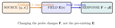
“电荷 \(Q\) 对电荷 \(q\) 施力”可以拆成两个彼此独立的问题:
\[\boxed{\text{source charges}\longrightarrow \mathbf E(\mathbf r)} \qquad \boxed{\mathbf E(\mathbf r)\longrightarrow \mathbf F=q\mathbf E}.\]
第一步只由源电荷及其状态决定;第二步才放入某个受力电荷。这样,一旦空间中的场已经求出,同一点放入不同的电荷便不必重新计算所有源的 Coulomb 力。12
0.2 One source point, one field point, one separation vector
全课固定使用以下记号:
| Symbol | 中文含义 | Role / 作用 |
|---|---|---|
| \(\mathbf r'\) | 源点位置 | 电荷元 \(dq\) 所在位置;积分变量 |
| \(\mathbf r\) | 场点位置 | 要计算电场的位置;积分时保持固定 |
| \(\mathbf R=\mathbf r-\mathbf r'\) | 从源点指向场点的分离矢量 | 决定 Coulomb 场的方向与距离 |
| \(R=\lvert\mathbf R\rvert\) | 源点到场点的距离 | 出现在反平方因子中 |
| \(\widehat{\mathbf R}=\mathbf R/R\) | 分离方向单位矢量 | 正源电荷的场方向 |
| \(q_0\) | 试探电荷 | 用来定义或测量场,最终取弱扰动极限 |
| \(k_e=1/(4\pi\varepsilon_0)\) | Coulomb 常量 | \(8.987\,551\,786\times10^9\ \mathrm{N\,m^2/C^2}\) |
在 SI 中,
\[[\mathbf E]=\mathrm{N/C}.\]
后续电势课会证明它也可写成 \(\mathrm{V/m}\),但本课只需从 \(\mathbf F=q\mathbf E\) 得到 \(\mathrm{N/C}\)。
Knowledge 1 — Test-charge and operational definition of electric field / 电场的试探电荷定义
Knowledge ID: P04-U01-L02-K01
1.1 Definition as a limiting measurement
在选定参考系中,把一个正的、点状、足够小并瞬时静止的试探电荷 \(q_0\) 放在场点 \(\mathbf r\)。测量其他电荷对它的电力 \(\mathbf F_{\rm ext}\),定义
\[\boxed{ \mathbf E(\mathbf r) =\lim_{q_0\to0^+} \frac{\mathbf F_{\rm ext}(\mathbf r;q_0)}{q_0} }.\]
“\(q_0\to0^+\)”同时编码了两件事:
- \(q_0>0\) 固定电场方向为正试探电荷受力方向;
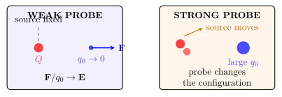
- 取弱探针极限,使探针不显著移动、极化或重排源电荷。
若源不受探针影响,则在足够小的区间
\[\mathbf F_{\rm ext}=q_0\mathbf E,\]
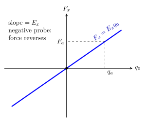
因此某一分量的 \(F\)–\(q_0\) 图像斜率就是对应的电场分量。
1.2 Why the field is independent of the probe
假设同一点依次放入 \(+q_a\)、\(+q_b\) 和 \(-q_a\),且三者都不扰动源:
\[\frac{\mathbf F_a}{q_a} =\frac{\mathbf F_b}{q_b} =\frac{\mathbf F_{-a}}{-q_a} =\mathbf E(\mathbf r).\]
负电荷所受力与 \(\mathbf E\) 反向,但除以带符号的负电荷后,仍得到同一个 \(\mathbf E\)。因此“用正试探电荷”是规定方向的便利,不表示只有正电荷能测场。
1.3 Operational boundary conditions
真实测量永远不是一个抽象极限。定义成立需要逐项说明以下边界:
| Boundary / 边界 | Required condition | If violated |
|---|---|---|
| 弱扰动 | 探针产生的场远小于待测场,且不重排源 | 测到的是“源 + 探针”耦合后的新系统 |
| 点探针 | 探针尺寸 \(\ell\ll L_E\),其中 \(L_E\) 是场的变化尺度 | 测到有限体积平均,而非单点值 |
| 排除自场 | \(\mathbf F_{\rm ext}\) 只含其他源对探针的力 | 点电荷自场在自身位置发散,不能代入 \(q\mathbf E_{\rm self}\) |
| 瞬时静止 | 用 \(\mathbf v=0\) 的探针,或已扣除磁力 \(q\mathbf v\times\mathbf B\) | 运动探针的总 Lorentz 力不再只等于 \(q\mathbf E\) |
| 指定参考系 | \(\mathbf r,t\) 和“静止”均相对某惯性系 | 电场与磁场在不同参考系会混合 |
| 外力分离 | 重力、接触力等已单独扣除 | \(\mathbf F_{\rm total}/q\) 不是电场 |
1.4 Static definition and the general electromagnetic caveat
本课讨论静电场。更一般地,带电粒子的电磁力为
\[\mathbf F_{\rm em}=q(\mathbf E+\mathbf v\times\mathbf B).\]
所以要用受力定义单独识别 \(\mathbf E\),最干净的方案是令试探电荷在测量瞬间 \(\mathbf v=0\)。在强时间变化、辐射或量子尺度下,探针反作用与“点粒子”模型还需更高级理论;这些不改变本课的静电定义,但限制它的实验实现。
Knowledge 2 — Electric field of point charges / 点电荷电场
Knowledge ID: P04-U01-L02-K02
2.1 One point source in vector form
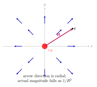
源电荷 \(q\) 位于 \(\mathbf r'\)。在场点 \(\mathbf r\ne\mathbf r'\),分离矢量为
\[\mathbf R=\mathbf r-\mathbf r', \qquad R=|\mathbf R|, \qquad \widehat{\mathbf R}=\frac{\mathbf R}{R}.\]
由 Coulomb 定律除以试探电荷,得到
\[\boxed{ \mathbf E_q(\mathbf r) =k_e\frac{q}{R^2}\widehat{\mathbf R} =k_e q\frac{\mathbf r-\mathbf r'}{|\mathbf r-\mathbf r'|^3} }.\]
方向信息已经包含在带符号的 \(q\) 中:
- \(q>0\):\(\mathbf E\) 沿 \(\widehat{\mathbf R}\),从源点向外;
- \(q<0\):\(\mathbf E\) 与 \(\widehat{\mathbf R}\) 反向,指向源点。
2.2 Inverse-square structure and unit check
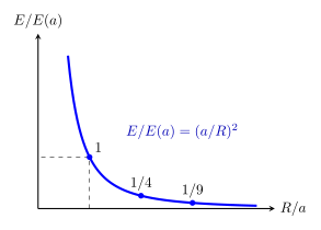
大小满足
\[E(R)=k_e\frac{|q|}{R^2}.\]
距离加倍,场强变为四分之一;距离乘三,场强变为九分之一。量纲为
\[[E] =\frac{\mathrm{N\,m^2}}{\mathrm{C^2}} \frac{\mathrm C}{\mathrm{m^2}} =\mathrm{N/C}.\]
2.3 Superposition for many point charges
若有 \(N\) 个点电荷 \(q_i\) 位于 \(\mathbf r_i'\),每个源独立贡献一个场,净场为矢量和:
\[\boxed{ \mathbf E(\mathbf r) =\sum_{i=1}^{N}\mathbf E_i(\mathbf r) =k_e\sum_{i=1}^{N} q_i\frac{\mathbf r-\mathbf r_i'}{|\mathbf r-\mathbf r_i'|^3} }.\]
可靠的计算顺序是:
- 对每个源写 \(\mathbf R_i=\mathbf r-\mathbf r_i'\);
- 单独求 \(\mathbf E_i\) 的方向和大小;
- 分解成同一坐标系中的分量;
- 分量相加;
- 最后才求净场大小和方向。
2.4 Worked Example 1 — a fully vectorial two-source field
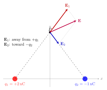
取
\[q_1=+2.00\ \mathrm{nC},\quad \mathbf r_1'=(-0.030,0)\ \mathrm m,\]
\[q_2=-1.00\ \mathrm{nC},\quad \mathbf r_2'=(+0.030,0)\ \mathrm m,\]
并求 \(P=(0,0.040)\ \mathrm m\) 处的电场。两源到 \(P\) 的距离均为 \(0.050\ \mathrm m\):
\[\widehat{\mathbf R}_1=0.6\widehat{\mathbf x}+0.8\widehat{\mathbf y},\]
而负电荷的场在 \(P\) 指向 \(q_2\):
\[\mathbf E_1 =7.190\times10^3(0.6\widehat{\mathbf x}+0.8\widehat{\mathbf y})\]
\[=(4.314\widehat{\mathbf x}+5.752\widehat{\mathbf y})\times10^3\ \mathrm{N/C},\]
\[\mathbf E_2 =3.595\times10^3(0.6\widehat{\mathbf x}-0.8\widehat{\mathbf y})\]
\[=(2.157\widehat{\mathbf x}-2.876\widehat{\mathbf y})\times10^3\ \mathrm{N/C}.\]
因此
\[\boxed{ \mathbf E =(6.471\widehat{\mathbf x}+2.876\widehat{\mathbf y})\times10^3\ \mathrm{N/C} }\]
\[\boxed{ E=7.081\times10^3\ \mathrm{N/C}, \qquad \theta=23.96^\circ\ \text{above }+x }.\]
2.5 Symmetry can cancel components—or the whole field
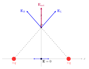
两个相同正电荷位于 \(x=\pm a\)。在垂直平分线上的点 \((0,y)\),水平分量相消、竖直分量相加;在中点 \((0,0)\),两者全部相消。
Knowledge 3 — Field lines and vector-field representation / 电场线与矢量场表示
Knowledge ID: P04-U01-L02-K03
3.1 The electric field is a vector field
在固定时刻,电场把空间中的每个允许场点映射到一个矢量:
\[\mathbf E:\ \mathbf r\longmapsto\mathbf E(\mathbf r).\]
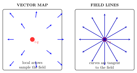
一个**矢量场图(vector-field map)**在许多采样点画出箭头:
- 箭头方向表示局部 \(\mathbf E\) 的方向;
- 若图例明确,箭头长度可表示 \(E\) 的相对大小;
- 由于真实场在每一点都有值,有限数量的箭头只是采样,而不是场本身。
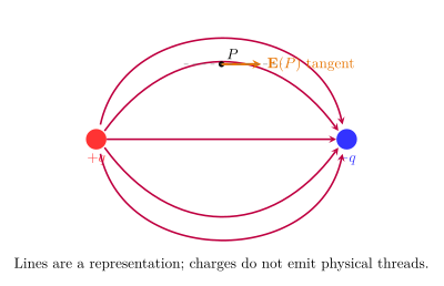
一个**电场线图(electric-field-line diagram)**则画出一族曲线,使任一点的曲线切线与局部电场同向。若曲线写成 \(\mathbf r(s)\),可用
\[\boxed{ \frac{d\mathbf r}{ds}\parallel\mathbf E[\mathbf r(s)] }\]
表达;若 \(s\) 选作弧长,还可写成
\[\frac{d\mathbf r}{ds}=\frac{\mathbf E}{|\mathbf E|}.\]
电场线的形状编码方向,但参数 \(s\) 不是时间,曲线上“走多快”也不等于粒子的实际速度。34
3.2 Rules for electrostatic field lines
在本课的静电范围内,一幅自洽的场线图遵守:
- 场线从正电荷或无穷远出发,终止于负电荷或无穷远;
- 箭头沿正试探电荷受力方向,从“\(+\)”指向“\(-\)”;
- 每一点的 \(\mathbf E\) 与通过该点的场线相切;
- 在同一幅图采用一致画法时,场线越密表示场越强;
- 从某电荷出发或终止的线数可按 \(|q|\) 的相对大小分配;
- 场线不能在 \(\mathbf E\ne0\) 的普通点相交;
- 静电场线不形成闭合回路。
第 4、5 条是表示约定而不是新的测量定律:画 8 条还是 16 条都可以,只要同图比例一致。没有图例时,不能从纸面线距读出精确的 \(\mathrm{N/C}\) 数值。OpenStax 与 Feynman 的表述都强调,线密度代表的是穿过垂直截面的线数/面积,而非沿曲线方向的“一维间距”。34
3.3 Why field lines cannot cross
若两条场线在一个普通点相交,它们给出的两条切线方向不同;于是同一点的 \(\mathbf E\) 将有两个方向,这与“场是单值矢量函数”矛盾。
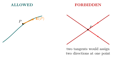
在 \(\mathbf E=0\) 的零点,方向本身未定义,场线的局部拓扑可能看起来像“分叉”或分隔区,但仍不能把它解释为一个非零矢量有两个方向。
3.4 Field lines are not particle trajectories
场线只回答“若在这一点瞬时放入正、静止试探电荷,它的加速度指向哪里”。真实轨迹还取决于:
- 粒子的初速度;
- 电荷正负号;
- 惯性与到达新位置所需时间;
- 场随位置和时间的变化;
- 其他力。
因此,负电荷从静止释放会向场线箭头反向加速;带横向初速度的正电荷即使在匀强场中也走抛物线,而不是沿一条直场线。
3.5 Reading a representation without over-reading it
| What the diagram supports | What it does not support without extra data |
|---|---|
| 某点的场方向 | 精确场强数值 |
| 同图中强弱的定性比较 | 不同作者图之间按线数直接比较 |
| 对称轴与零场候选区 | 默认把场线当作粒子路径 |
| 源汇位置与相对电荷量 | 把离散画出的线当作真实物体 |
Knowledge 4 — Motion of a charge in a uniform electric field / 电荷在匀强电场中的运动
Knowledge ID: P04-U01-L02-K04
4.1 Uniform field and the force direction
匀强电场(uniform electric field)是在所研究区域内大小和方向都不随位置改变的场:
\[\mathbf E(\mathbf r)=\mathbf E_0.\]
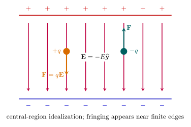
两块面积远大于间距的相反带电平行板,在远离边缘的中央区域近似产生匀强场。若理想无限薄板面电荷密度为 \(+\sigma\) 与 \(-\sigma\),单板每侧场强为 \(\sigma/(2\varepsilon_0)\);叠加后板间
\[E=\frac{\sigma}{\varepsilon_0},\]
板外则相消。此处把单板结果作为后续 Gauss-law lesson 的前瞻结论,不在本课用它替代 Coulomb 主线。
4.2 Derivation from Newton's second law
若只有给定外电场施加电力,
\[m\frac{d^2\mathbf r}{dt^2}=q\mathbf E_0.\]
于是加速度为常矢量
\[\boxed{\mathbf a=\frac{q}{m}\mathbf E_0}.\]
积分一次和两次:
\[\boxed{ \mathbf v(t)=\mathbf v_0+\frac{q\mathbf E_0}{m}t }\]
\[\boxed{ \mathbf r(t)=\mathbf r_0+\mathbf v_0t +\frac12\frac{q\mathbf E_0}{m}t^2 }.\]
质量只影响加速度大小,电荷符号控制加速度相对 \(\mathbf E\) 的方向。响应尺度由荷质比 \(q/m\) 决定。
4.3 Perpendicular injection gives a parabola
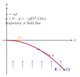
令
\[\mathbf E=E\widehat{\mathbf y}, \qquad \mathbf v_0=v_0\widehat{\mathbf x}, \qquad \mathbf r_0=(0,0).\]
则
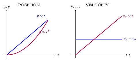
\[x=v_0t, \qquad y=\frac{qE}{2m}t^2.\]
消去 \(t=x/v_0\):
\[\boxed{ y(x)=\frac{qE}{2mv_0^2}x^2 }.\]
这是抛物线。若 \(q<0\),开口与 \(\mathbf E\) 相反;若还有非零 \(v_{0y}\),则再加线性项 \((v_{0y}/v_{0x})x\)。
4.4 Position and velocity as functions of time
横向运动保持匀速,而场方向速度线性变化、位移二次变化:
4.5 Worked Example 2 — electron beam between plates
一个电子以
\[v_0=5.00\times10^6\ \mathrm{m/s}\]
沿 \(+x\) 方向进入长度 \(L=2.00\ \mathrm{cm}\) 的匀强电场区,
\[\mathbf E=+1.50\times10^3\ \mathrm{N/C}\,\widehat{\mathbf y}.\]
采用 \(e=1.602\,176\,634\times10^{-19}\ \mathrm C\) 与 \(m_e=9.109\,383\,71\times10^{-31}\ \mathrm{kg}\),电子 \(q=-e\)。56
横向飞行时间:
\[t=\frac{L}{v_0} =\frac{0.0200}{5.00\times10^6} =4.00\times10^{-9}\ \mathrm s.\]
竖直加速度:
\[a_y=\frac{-eE}{m_e} =-2.638\times10^{14}\ \mathrm{m/s^2}.\]
出口偏转与竖直速度:
\[\boxed{ y=\frac12a_yt^2=-2.111\times10^{-3}\ \mathrm m }\]
\[\boxed{ v_y=a_yt=-1.055\times10^6\ \mathrm{m/s} }.\]
出口速率和方向为
\[v=5.110\times10^6\ \mathrm{m/s}, \qquad \theta=-11.92^\circ.\]
由于 \(v/c\approx0.0170\ll1\),非相对论近似自洽。负号表示电子向电场反方向偏转。
4.6 Model boundary
本节解法要求:
- 电场在粒子经过的整个区域近似恒定;
- 电场由外部装置给定,单粒子不显著改变它;
- 忽略磁场、重力、碰撞与其他粒子相互作用;
- 忽略辐射损失和自身反作用;
- \(v\ll c\),可用 Newton 力学;
- 平行板近似只用于板宽远大于间距且远离边缘的中央区域。
若任一条件失败,\(\mathbf a=q\mathbf E/m\) 可能随位置、时间或速度变化,简单抛物线不再成立。
Knowledge 5 — Continuous charge distributions / 连续电荷分布
Knowledge ID: P04-U01-L02-K05
5.1 Continuum is a controlled macroscopic approximation
电荷量子化意味着真实物质由离散电荷组成;“连续带电体”并非声称电荷可以任意分割。它的含义是:选取一个尺度很小的电荷元,其中仍含有许多微观电荷,同时该尺度又远小于几何尺寸和场的变化尺度。于是可用平滑密度函数代替逐粒子求和。78
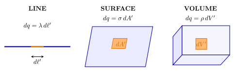
三类常用密度为
\[\boxed{\lambda(\mathbf r')=\frac{dq}{d\ell'}} \qquad [\lambda]=\mathrm{C/m},\]
\[\boxed{\sigma(\mathbf r')=\frac{dq}{dA'}} \qquad [\sigma]=\mathrm{C/m^2},\]
\[\boxed{\rho(\mathbf r')=\frac{dq}{dV'}} \qquad [\rho]=\mathrm{C/m^3}.\]
相应的电荷元与总电荷为
\[dq=\lambda\,d\ell', \qquad Q=\int_{\rm line}\lambda(\mathbf r')\,d\ell',\]
\[dq=\sigma\,dA', \qquad Q=\iint_{\rm surface}\sigma(\mathbf r')\,dA',\]
\[dq=\rho\,dV', \qquad Q=\iiint_{\rm volume}\rho(\mathbf r')\,dV'.\]
5.2 From a discrete sum to the master integral
离散点电荷的场为
\[\mathbf E(\mathbf r) =k_e\sum_i q_i \frac{\mathbf r-\mathbf r_i'}{|\mathbf r-\mathbf r_i'|^3}.\]
把足够小的电荷元 \(dq\) 当作点电荷,并令分割趋于连续,Riemann 和变成
\[d\mathbf E(\mathbf r) =k_e\,dq\, \frac{\mathbf R}{R^3}, \qquad \mathbf R=\mathbf r-\mathbf r'.\]
因此主公式是
\[\boxed{ \mathbf E(\mathbf r) =k_e\int \frac{\mathbf r-\mathbf r'}{|\mathbf r-\mathbf r'|^3}\,dq(\mathbf r') }.\]
分别代入三种密度:
\[\boxed{ \mathbf E_{\rm line}(\mathbf r) =k_e\int_{\rm line} \lambda(\mathbf r') \frac{\mathbf r-\mathbf r'}{|\mathbf r-\mathbf r'|^3}\,d\ell' }\]
\[\boxed{ \mathbf E_{\rm surface}(\mathbf r) =k_e\iint_{\rm surface} \sigma(\mathbf r') \frac{\mathbf r-\mathbf r'}{|\mathbf r-\mathbf r'|^3}\,dA' }\]
\[\boxed{ \mathbf E_{\rm volume}(\mathbf r) =k_e\iiint_{\rm volume} \rho(\mathbf r') \frac{\mathbf r-\mathbf r'}{|\mathbf r-\mathbf r'|^3}\,dV' }.\]
这些是矢量积分。写成 \(\int k_e\,dq/R^2\) 只给出每个微元场的大小;除非所有 \(d\mathbf E\) 同向,否则还必须投影分量。
5.3 A five-step integration workflow
- Geometry: 画源、场点、\(\mathbf r'\)、\(\mathbf r\)、\(\mathbf R\);
- Element: 选 \(dq=\lambda d\ell'\)、\(dq=\sigma dA'\) 或 \(dq=\rho dV'\);
- Symmetry: 在积分前判定必为零或成对抵消的分量;
- One variable system: 把 \(R\)、方向余弦和 \(dq\) 全改写成同一组积分变量;
- Checks: 检查单位、方向、远场、特殊点和无限尺寸极限。
5.4 Derivation — finite uniformly charged segment
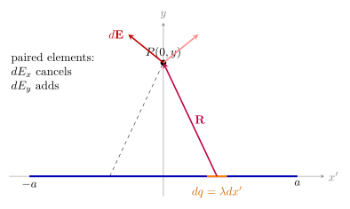
一根均匀细杆位于 \(x'\) 轴,范围 \(-a\le x'\le a\),线密度为常量 \(\lambda>0\)。求场点
\[\mathbf r=(0,y),\qquad y>0\]
处的场。源点、电荷元与分离矢量为
\[\mathbf r'=x'\widehat{\mathbf x}, \qquad dq=\lambda\,dx',\]
\[\mathbf R =-x'\widehat{\mathbf x}+y\widehat{\mathbf y}, \qquad R=\sqrt{x'^2+y^2}.\]
微元场为
\[d\mathbf E =k_e\lambda\,dx' \frac{-x'\widehat{\mathbf x}+y\widehat{\mathbf y}} {(x'^2+y^2)^{3/2}}.\]
\(x'\) 与 \(-x'\) 的 \(x\) 分量相消,故
\[E_x=0,\]
\[E_y =2k_e\lambda y \int_0^a\frac{dx'}{(x'^2+y^2)^{3/2}}.\]
利用
\[\int\frac{dx'}{(x'^2+y^2)^{3/2}} =\frac{x'}{y^2\sqrt{x'^2+y^2}},\]
得到
\[\boxed{ \mathbf E(0,y) =\frac{2k_e\lambda a}{y\sqrt{a^2+y^2}} \widehat{\mathbf y} }.\]
因总电荷 \(Q=2a\lambda\),也可写成
\[\mathbf E(0,y) =\frac{k_eQ}{y\sqrt{a^2+y^2}}\widehat{\mathbf y}.\]
两个重要极限同时检验结果:
\[y\gg a: \quad \mathbf E\simeq\frac{k_eQ}{y^2}\widehat{\mathbf y} \quad\text{(far field: point charge)},\]
\[a\to\infty\ \text{at fixed }\lambda: \quad \mathbf E\to\frac{2k_e\lambda}{y}\widehat{\mathbf y} =\frac{\lambda}{2\pi\varepsilon_0y}\widehat{\mathbf y}.\]
5.5 Derivation — uniformly charged ring on its axis
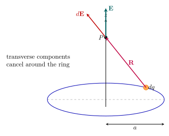
半径为 \(a\)、总电荷为 \(Q\) 的均匀圆环位于 \(xy\) 平面,场点为 \(\mathbf r=z\widehat{\mathbf z}\)。任一电荷元到场点的距离都为
\[R=\sqrt{a^2+z^2}.\]
对径微元的横向分量相消,只有 \(z\) 分量相加。对每个微元,
\[dE_z =\left(k_e\frac{dq}{a^2+z^2}\right) \frac{z}{\sqrt{a^2+z^2}}.\]
由于分母和方向余弦对全环相同,
\[\boxed{ \mathbf E(z) =k_e\frac{Qz}{(z^2+a^2)^{3/2}} \widehat{\mathbf z} }.\]
该结果给出三个高价值检查:
\[E_z(0)=0,\]
\[z\gg a: \quad E_z\simeq k_e\frac{Q}{z^2},\]
\[z\ll a: \quad E_z\simeq k_e\frac{Q}{a^3}z.\]
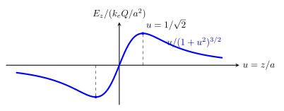
最后一个近轴结果说明中心附近的场对 \(z\) 近似线性。对
\[\frac{z}{(z^2+a^2)^{3/2}}\]
求导可得极值条件 \(a^2-2z^2=0\)。若 \(Q>0\),正轴上的场强最大值位于
\[\boxed{z=\frac{a}{\sqrt2}},\]
且
\[|E|_{\max} =\frac{2}{3\sqrt3}\frac{k_e|Q|}{a^2}.\]
5.6 Surface distribution — disk as concentric rings
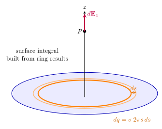
半径为 \(R_0\)、均匀面密度为 \(\sigma\) 的圆盘可分解为半径 \(s\)、宽度 \(ds\) 的同心细环:
\[dq=\sigma(2\pi s\,ds).\]
在正轴 \(z>0\) 上,代入圆环轴线场:
\[dE_z =k_e\frac{z\,dq}{(z^2+s^2)^{3/2}} =2\pi k_e\sigma z \frac{s\,ds}{(z^2+s^2)^{3/2}}.\]
积分 \(s:0\to R_0\):
\[E_z =2\pi k_e\sigma z \int_0^{R_0} \frac{s\,ds}{(z^2+s^2)^{3/2}},\]
\[\boxed{ \mathbf E(z) =\frac{\sigma}{2\varepsilon_0} \left(1-\frac{z}{\sqrt{z^2+R_0^2}}\right) \widehat{\mathbf z}, \qquad z>0 }.\]
极限检查:
\[z\gg R_0: \quad E_z\simeq k_e\frac{\sigma\pi R_0^2}{z^2} =k_e\frac{Q}{z^2},\]
\[R_0\to\infty: \quad E_z\to\frac{\sigma}{2\varepsilon_0}.\]
5.7 Volume distribution — the exact setup
对一般体密度,选择与几何相适配的体积元。例如球坐标源点
\[\mathbf r'=s\widehat{\mathbf r}', \qquad dV'=s^2\sin\theta'\,ds\,d\theta'\,d\phi'.\]
若场点选在 \(z\) 轴 \(\mathbf r=z\widehat{\mathbf z}\),则严格的 Coulomb 积分是
\[\boxed{ \mathbf E(z\widehat{\mathbf z}) =k_e \int \rho(s,\theta',\phi') \frac{z\widehat{\mathbf z}-s\widehat{\mathbf r}'} {(z^2+s^2-2zs\cos\theta')^{3/2}} s^2\sin\theta'\,ds\,d\theta'\,d\phi' }.\]
本式明确展示:即使 \(\rho\) 为常量,方向矢量和距离仍随三个源坐标变化。对高度对称分布,Gauss 定律课 会显著缩短计算;但它不会改变这里的源点—场点结构。
6. Lesson synthesis / 全课整合
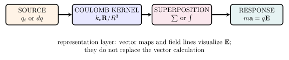
6.1 One chain from source to motion
6.2 Core equation sheet
6.3 A diagnostic workflow for any electric-field problem
- System boundary: 哪些是源?哪个电荷只是受力对象?
- Model: 点电荷、离散多源、连续线/面/体,还是给定匀强外场?
- Coordinates: 固定 \(\mathbf r\),参数化 \(\mathbf r'\),写 \(\mathbf R=\mathbf r-\mathbf r'\)。
- Direction sketch: 先画每个 \(d\mathbf E\) 或 \(\mathbf E_i\) 的方向。
- Symmetry: 哪些分量必为零?哪些成对相加?
- Calculate: 离散用 \(\sum\),连续用 \(\int\);只在最后求大小。
- Respond: 若问受力或运动,再用 \(\mathbf F=q\mathbf E\) 与 Newton 定律。
- Audit: 单位、符号、极限、近似尺度与是否误加自场。
6.4 Approximation map
| Model | Reliable when | Main failure signal |
|---|---|---|
| 试探电荷 | 探针弱、小、可分离外力 | 源随探针明显重排 |
| 点电荷 | 源尺寸远小于 \(R\) | 场点接近或进入有限源内部 |
| 连续分布 | 每个宏观微元含许多电荷 | 距离接近粒子间距或密度剧烈离散 |
| 无限线/面 | 端部尺度远大于观察距离 | 接近边缘或与整体尺寸同量级 |
| 匀强场运动 | \(\mathbf E\) 恒定、\(v\ll c\)、外场给定 | 边缘场、相对论、碰撞或反作用显著 |
| 场线图 | 只需方向和相对强弱 | 把图上线数当成精确测量 |
7. Misconception clinic / 易错概念诊所
| Misconception / 错误观念 | Correction / 修正 |
|---|---|
| “电场是单位正电荷受到的力,所以必须真的放一个 \(1\ \mathrm C\) 电荷。” | \(1\ \mathrm C\) 通常巨大并会严重扰动源;定义是 \(q_0\to0^+\) 的比值极限。 |
| “负试探电荷测得相反的电场。” | 它受相反的力;除以带符号的负电荷仍得同一 \(\mathbf E\)。 |
| “一个电荷受到自己产生的 \(k_eq/r^2\) 场。” | 本课粒子受力用外场,不把理想点电荷发散的自场加入。 |
| “零净场表示该点没有任何源贡献。” | 多个非零矢量可以相消。 |
| “叠加就是把 \(E_1,E_2\) 的大小相加。” | 叠加的是矢量或其坐标分量。 |
| “场线就是电荷实际走过的轨迹。” | 场线是瞬时局部方向图;轨迹还依赖初速度、惯性与电荷符号。 |
| “场线越多,实际空间里就有越多条东西。” | 场线是人为选择的连续场表示,不是物理丝线。 |
| “场线交叉只是图画得密。” | 非零场点若交叉会给一个点两个方向,物理上不自洽。 |
| “点电荷场在源点无穷大,所以任何真实带电体表面也无穷大。” | 发散属于零尺寸点源理想化;有限分布必须积分并使用适当内部模型。 |
| “匀强电场中的粒子一定沿直线运动。” | 有横向初速度时为抛物线;只有速度与加速度共线时才是一维直线。 |
| “连续电荷违反电荷量子化。” | 它是许多离散电荷在宏观尺度上的受控平均。 |
| “\(r\) 在连续积分里始终是同一个距离。” | \(\mathbf r\) 固定、\(\mathbf r'\) 变化,因此 \(R=\lvert\mathbf r-\mathbf r'\rvert\) 一般随积分变量变化。 |
| “无限平面给常量场与反平方定律矛盾。” | 每个微元仍服从反平方;距离增大时参与贡献的有效面积也增大,积分后产生不同标度。 |
8. Practice and retrieval / 练习与检索
A. Conceptual questions
- 为什么操作定义写 \(q_0\to0^+\),而不是直接令 \(q_0=0\)?
- 能否用负试探电荷测电场?需要怎样处理方向?
- 两个正电荷连线上的零场点是否一定在两者之间?若两电荷大小不同,零点是否仍在中点?
- 为什么电场线不相交?若某点 \(\mathbf E=0\),这个论证的哪一步不再适用?
- 一粒负电荷从静止释放时,它沿电场线箭头还是反箭头加速?
- 有横向初速度的带电粒子在匀强电场中为什么不是沿场线运动?
- 连续分布积分中,为什么必须区分 \(\mathbf r\) 与 \(\mathbf r'\)?
- 一个有限圆盘在什么极限下像点电荷?在什么极限下像无限平面?
- 对称分布是否自动意味着场为零?请给一个“只消去部分分量”的例子。
- 为什么用无限线或无限面模型时,必须同时说明观察距离与物体尺寸的比较?
B. Quantitative and derivation questions
- 一个点电荷 \(q=-4.00\ \mathrm{nC}\) 位于原点。求 \(P=(3.00,4.00)\ \mathrm{cm}\) 处的电场矢量。
- 两个 \(+2.00\ \mathrm{nC}\) 点电荷位于 \((\pm3.00\ \mathrm{cm},0)\)。求 \(P=(0,4.00\ \mathrm{cm})\) 处的净电场。
- 一个质子从静止释放在 \(E=2.50\times10^3\ \mathrm{N/C}\) 的匀强场中。取 \(m_p=1.672\,621\,925\,95\times10^{-27}\ \mathrm{kg}\),忽略其他力,求 \(20.0\ \mathrm{ns}\) 后的速率与位移。
- 均匀带电细杆范围为 \(-0.120\le x'\le0.120\ \mathrm m\),\(\lambda=4.00\ \mathrm{nC/m}\)。求 \((0,0.160\ \mathrm m)\) 处的场。
- 均匀圆环 \(Q=3.00\ \mathrm{nC}\)、\(a=5.00\ \mathrm{cm}\)。求 \(z=5.00\ \mathrm{cm}\) 处的轴向场,并说明方向。
- 证明圆环轴线场在 \(z=a/\sqrt2\) 达到正轴最大值,并求归一化最大值 \(E_{\max}/(k_eQ/a^2)\)。
- 均匀圆盘 \(\sigma=1.20\ \mu\mathrm{C/m^2}\)、\(R_0=8.00\ \mathrm{cm}\)。求正轴 \(z=3.00\ \mathrm{cm}\) 处的场。
- 从有限细杆结果出发,分别取 \(y\gg a\) 与 \(a\to\infty\),恢复点电荷和无限长线的结果。
Answers / 参考答案
1. \(q_0=0\) 时力也为零,无法形成可测比值;极限表示用越来越弱的探针外推,同时消除源的扰动。
2. 可以。负探针受力与 \(\mathbf E\) 反向,但必须除以带符号的 \(q_0<0\)。
3. 同号电荷的有限零点若存在于连线上,会在两者之间;大小不同则靠近较小电荷,不在中点。
4. 相交会在同一点给出两个切向方向;在 \(\mathbf E=0\) 点,单位方向 \(\mathbf E/E\) 未定义。
5. 反箭头。
6. 电场只改变场方向速度分量,横向初速度因惯性保留,合成轨迹为抛物线。
7. \(\mathbf r\) 是固定场点,\(\mathbf r'\) 扫过源;若不区分,就会错误地把距离和方向当作常量。
8. \(z\gg R_0\) 时像总电荷集中的点源;\(R_0\gg z\) 且远离边缘时像无限平面。
9. 不自动。均匀细杆垂直平分线上的场,水平分量相消而竖直分量相加。
10. “无限”是局部尺度近似;若观察距离可见端部,所得 \(1/r\) 或常量场不再可靠。
11. \(R=5.00\ \mathrm{cm}\),方向指向原点:
\[\mathbf E=(-8.628\widehat{\mathbf x}-11.504\widehat{\mathbf y})\times10^3\ \mathrm{N/C},\]
\[E=1.438\times10^4\ \mathrm{N/C}.\]
12. 水平分量相消,每个场的竖直分量为 \(7.190\times10^3(0.8)\):
\[\mathbf E=1.150\times10^4\ \mathrm{N/C}\,\widehat{\mathbf y}.\]
13.
\[a=\frac{eE}{m_p}=2.394\times10^{11}\ \mathrm{m/s^2},\]
\[v=4.789\times10^3\ \mathrm{m/s},
\qquad
\Delta x=4.789\times10^{-5}\ \mathrm m.\]
14. \(a=0.120\ \mathrm m\)、\(y=0.160\ \mathrm m\)、\(\sqrt{a^2+y^2}=0.200\ \mathrm m\):
\[\mathbf E
=\frac{2k_e\lambda a}{y\sqrt{a^2+y^2}}\widehat{\mathbf y}
=2.696\times10^2\ \mathrm{N/C}\,\widehat{\mathbf y}.\]
15.
\[\mathbf E
=k_e\frac{Qz}{(z^2+a^2)^{3/2}}\widehat{\mathbf z}
=3.813\times10^3\ \mathrm{N/C}\,\widehat{\mathbf z}.\]
16.
\[\frac{d}{dz}\frac{z}{(z^2+a^2)^{3/2}}
=\frac{a^2-2z^2}{(z^2+a^2)^{5/2}}=0,\]
故 \(z=a/\sqrt2\);
\[\frac{E_{\max}}{k_eQ/a^2}=\frac{2}{3\sqrt3}=0.3849.\]
17.
\[\mathbf E
=\frac{\sigma}{2\varepsilon_0}
\left(1-\frac{z}{\sqrt{z^2+R_0^2}}\right)\widehat{\mathbf z}
=4.40\times10^4\ \mathrm{N/C}\,\widehat{\mathbf z}.\]
18. \(y\gg a\) 时 \(\sqrt{a^2+y^2}\simeq y\),且 \(Q=2a\lambda\),故 \(E\simeq k_eQ/y^2\);\(a\to\infty\) 时 \(a/\sqrt{a^2+y^2}\to1\),故 \(E\to2k_e\lambda/y=\lambda/(2\pi\varepsilon_0y)\)。
Exit ticket
不查公式,用四句话回答:
- 电场怎样从力定义出来,为什么需要弱探针极限?
- 多个源的场怎样组合?
- 场线与粒子轨迹的根本区别是什么?
- 离散求和怎样推广为连续分布积分?
Exit-ticket benchmark
电场是外源对正、点状、弱试探电荷的受力/电荷极限,弱探针保证不改变源;多个源的贡献按矢量叠加;场线是处处与瞬时电场相切的表示,而轨迹还由初速度、惯性和电荷符号决定;连续分布把 \(q_i\) 换成 \(dq=\lambda d\ell'\)、\(dq=\sigma dA'\) 或 \(dq=\rho dV'\),并对源位置 \(\mathbf r'\) 积分,同时保持场点 \(\mathbf r\) 固定。
9. References and source notes / 参考资料与使用说明
9.1 Source-to-content map
| Source | Used for |
|---|---|
| OpenStax, University Physics Volume 2, §5.4 Electric Field | field as a probe-independent vector property, point-charge field, direction, superposition, SI units |
| OpenStax, §5.5 Calculating Electric Fields of Charge Distributions | continuum approximation, \(\lambda/\sigma/\rho\), line/surface/volume integrals, finite rod, ring, disk and infinite-sheet limits |
| OpenStax, §5.6 Electric Field Lines | vector-map versus field-line representation, tangent and density rules, non-crossing and diagram limits |
| MIT OCW 8.02, Chapter 2 — Coulomb's Law | operational electric field, Coulomb vector form, force on a charge, uniform-field motion and continuous distributions |
| MIT OCW 8.02T — presentati_w01d2.pdf (Electric Fields and Continuous Charge Distributions) | undergraduate lesson sequencing, ring/disk decompositions and visualization cross-check |
| Feynman Lectures, Vol. II, Ch. 4 — Electrostatics | geometry of field lines, line density, relation to the vector field, and warning that superposition is easier algebraically than pictorially |
| NIST — 2022 CODATA elementary charge | exact elementary charge used in the electron-motion calculation |
| NIST — 2022 CODATA recommended constants | electron and proton masses and independent numerical verification |
| University of Colorado Boulder PhET — Charges and Fields | optional interactive verification of superposition, vector maps and equipotential/field representations |
9.2 Bibliographic notes
- Ling, S. J., Moebs, W., and Sanny, J. University Physics Volume 2. OpenStax, Rice University, 2016. Sections 5.4–5.6 form the principal undergraduate source spine.
- Belcher, J. W., Dourmashkin, P., and Liao, S.-B. “Chapter 2: Coulomb's Law.” MIT OpenCourseWare 8.02, Spring 2007. Used to cross-check notation, uniform-field motion and continuous-source examples.
- Feynman, R. P., Leighton, R. B., and Sands, M. The Feynman Lectures on Physics, Vol. II, Ch. 4. California Institute of Technology. Used for the geometric interpretation and limitations of field-line pictures.
- CODATA Task Group on Fundamental Constants. “CODATA Recommended Values of the Fundamental Physical Constants: 2022.” NIST. Numerical examples retain sufficient significant figures for the input data rather than copying every CODATA digit.
- PhET Interactive Simulations. “Charges and Fields.” University of Colorado Boulder. Suggested as a qualitative and numerical cross-check, not as a substitute for vector calculation.
9.3 Reading and simulation route
- 想系统练习离散与连续源:先读 OpenStax §5.4–5.5,再做 MIT 8.02 Chapter 2 的连续分布问题。
- 想检查场线直觉:使用 PhET Charges and Fields,同时手算若干采样点验证箭头。9
- 想把对称性升级为通量方法:Electric Flux。
- 想用标量而非逐分量积分求场:Electric Potential。
- 想研究点电荷组的远场结构:Electric Dipoles and Multipoles。
注释与参考文献
OpenStax, University Physics Volume 2, §5.4 “Electric Field”.
↩MIT OpenCourseWare 8.02, Chapter 2: Coulomb's Law.
↩OpenStax, University Physics Volume 2, §5.6 “Electric Field Lines”.
↩ ↩Caltech, The Feynman Lectures on Physics, Vol. II, Ch. 4 “Electrostatics”.
↩ ↩NIST, 2022 CODATA value: elementary charge.
↩NIST, CODATA Recommended Values of the Fundamental Physical Constants: 2022.
↩OpenStax, University Physics Volume 2, §5.5 “Calculating Electric Fields of Charge Distributions”.
↩MIT OpenCourseWare 8.02T, presentati_w01d2.pdf — Electric Fields and Continuous Charge Distributions.
↩University of Colorado Boulder, PhET “Charges and Fields”.
↩