
Learning objectives / 学习目标
完成本课后,你应能:
- 从微小盒子的六面通量推导 Cartesian divergence,并解释其坐标无关定义。
- 用散度定理及“体积任意”条件从积分 Gauss law 推得局部形式,也能反向恢复积分形式。
- 从给定 \(\mathbf E\) 计算 \(\rho\),或用对称性和局部方程检验候选场;区分局部源强与场值大小。
- 使用三维 Dirac delta 表示点、线、面电荷,并以测试函数/积分意义解释等式。
- 正确处理 \(\nabla\cdot(\hat{\mathbf r}/r^2)\) 在 \(r=0\) 的分布贡献。
Prerequisites / 先修知识
- Gauss's Law and Symmetry:积分形式与包围电荷。
- 多变量微积分:偏导数、体积分、散度定理。
- 能区分 ordinary function、piecewise-smooth field 与 distribution 的积分意义。
Scope, conventions, and notation
- 真空、宏观经典静电,SI 制;Catalog 标题采用 \(\epsilon_0\),本文数值常数统一排作 \(\varepsilon_0\),二者都表示同一个真空介电常数。
- \(\rho\) 是体电荷密度,单位 \(\mathrm{C/m^3}\);表面、线、点源可以作为 distributions 嵌入三维 \(\rho\)。
- \(\nabla\cdot\mathbf E\) 单位为 \(\mathrm{N\,C^{-1}m^{-1}}=\mathrm{V/m^2}\)。
- 对普通光滑场,等式逐点成立;对含奇点的场,必须按分布意义理解。
- 完整静电局部方程还包括 \(\nabla\times\mathbf E=0\);本课聚焦 Catalog 指定的 Gauss 局部形式。
Knowledge 1 — Divergence of electric field / 电场散度
Knowledge ID: P04-U02-L03-K01
1.1 Flux per shrinking volume
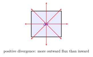
散度在点 \(\mathbf r\) 的坐标无关定义为
\[\boxed{ \nabla\cdot\mathbf E(\mathbf r) =\lim_{\Delta V\to0} \frac{1}{\Delta V} \oint_{\partial(\Delta V)}\mathbf E\cdot d\mathbf A }.\]
它衡量单位体积的净外向通量率。正散度像局部 source,负散度像 sink,零散度表示净流出为零——但不意味着场为零。
1.2 Cartesian derivation from a small box
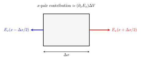
对中心在 \((x,y,z)\)、边长 \(\Delta x,\Delta y,\Delta z\) 的盒子,\(x\) 两面净通量近似
\[\left[E_x\left(x+\frac{\Delta x}{2}\right) -E_x\left(x-\frac{\Delta x}{2}\right)\right]\Delta y\Delta z \simeq\frac{\partial E_x}{\partial x}\Delta V.\]
三方向相加并除以 \(\Delta V\):
\[\boxed{ \nabla\cdot\mathbf E =\frac{\partial E_x}{\partial x} +\frac{\partial E_y}{\partial y} +\frac{\partial E_z}{\partial z} }.\]
Worked Example 1 — Infer local source density from a field
给定区域内
\[\mathbf E=\alpha(x\hat{\mathbf x}+2y\hat{\mathbf y}-z\hat{\mathbf z}), \qquad \alpha=4.00\times10^3\ \mathrm{V/m^2}.\]
- 研究区域: 场光滑的真空模型区域,Cartesian 坐标固定。
- 模型与方程: 由局部 Gauss law,\(\rho=\varepsilon_0\nabla\cdot\mathbf E\)。
- 计算:
\[\nabla\cdot\mathbf E=\alpha(1+2-1)=2\alpha,\]
\[\rho=2\varepsilon_0\alpha =\boxed{7.08\times10^{-8}\ \mathrm{C/m^3}}.\]
- 检查: 正号对应净源;量纲 \(\varepsilon_0(\mathrm{V/m^2})=\mathrm{C/m^3}\);把盒子各边同比缩小时,通量与体积同比缩小。
Knowledge 2 — Differential form \(\nabla\cdot\mathbf E=\rho/\epsilon_0\) / 高斯定律微分形式
Knowledge ID: P04-U02-L03-K02
2.1 From integral to local
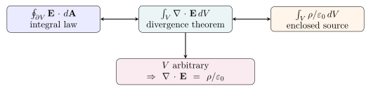
散度定理给出
\[\oint_{\partial V}\mathbf E\cdot d\mathbf A =\int_V\nabla\cdot\mathbf E\,dV.\]
与积分 Gauss law
\[\oint_{\partial V}\mathbf E\cdot d\mathbf A =\frac1{\varepsilon_0}\int_V\rho\,dV\]
比较,得到
\[\int_V\left(\nabla\cdot\mathbf E-\frac{\rho}{\varepsilon_0}\right)dV=0.\]
因为 \(V\) 是任意体积,光滑情形下被积函数逐点为零:
\[\boxed{\nabla\cdot\mathbf E=\frac{\rho}{\varepsilon_0}}.\]
2.2 From local back to integral
反向在任意体积积分并用散度定理:
\[\int_V\nabla\cdot\mathbf E\,dV =\frac1{\varepsilon_0}\int_V\rho\,dV \Longrightarrow \oint_{\partial V}\mathbf E\cdot d\mathbf A =\frac{Q_{\rm enc}}{\varepsilon_0}.\]
因此两种形式在适当正则性或 distribution 框架下等价;积分形式更自然地跨越不连续界面,局部形式更适合微分方程与数值场求解。
Worked Example 2 — Verify a spherically symmetric piecewise field
候选场
\[\mathbf E(r)= \begin{cases} Cr\,\hat{\mathbf r}, & r<R,\\ CR^3r^{-2}\hat{\mathbf r}, & r>R, \end{cases}\]
其中 \(C>0\)。判断对应体密度及 \(r=R\) 是否有表面电荷。
- 模型: 球坐标,\(r\ne0\);径向场散度
\[\nabla\cdot[E_r(r)\hat{\mathbf r}] =\frac1{r^2}\frac{d}{dr}(r^2E_r).\]
- 内部: \(r^2E_r=Cr^3\),故 \(\nabla\cdot\mathbf E=3C\),
\[\rho_{\rm in}=3\varepsilon_0C.\]
- 外部: \(r^2E_r=CR^3\),故 \(\rho_{\rm out}=0\)。
- 边界检查: \(E_r(R^-)=E_r(R^+)=CR\),法向场无跳跃,所以 \(\sigma=\varepsilon_0(E_{\rm out}-E_{\rm in})=0\)。
- 全局检查: 总电荷 \(4\pi R^3\varepsilon_0C\),外场恰为其 Coulomb 场。
Knowledge 3 — Charge density as a field source / 电荷密度作为场源
Knowledge ID: P04-U02-L03-K03
3.1 Local source does not mean local causation only
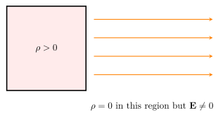
\(\rho(\mathbf r)\) 决定该点的散度,但 \(\mathbf E(\mathbf r)\) 本身由全空间电荷与边界条件共同决定。可能出现:
- \(\rho=0\) 但 \(\mathbf E\ne0\)(平行板之间、点电荷外部);
- \(\mathbf E=0\) at one point 但 \(\rho\ne0\)(均匀带电球中心);
- \(\nabla\cdot\mathbf E=0\) 但场空间变化显著(偶极远离源的区域)。
3.2 Density reconstruction and consistency checks
若实验或数值给出全矢量场,可计算
\[\rho=\varepsilon_0\nabla\cdot\mathbf E.\]
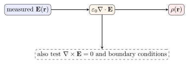
但静电候选场还必须满足 \(\nabla\times\mathbf E=0\)。仅满足 divergence 方程不能唯一确定矢量场,因为可叠加任意无散场;边界条件与 curl 方程共同完成约束。
Worked Example 3 — A field with zero divergence but nonzero curl
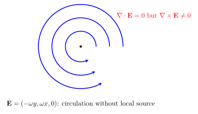
给定 \(\mathbf E=(-\omega y,\omega x,0)\),\(\omega\) 为常量。它能否是某单连通区域中的静电场?
- 局部源检查:
\[\nabla\cdot\mathbf E =\partial_x(-\omega y)+\partial_y(\omega x)=0,\]
所以若只看 Gauss 局部形式会得到 \(\rho=0\)。
- 静电完整性检查:
\[\nabla\times\mathbf E=(0,0,2\omega)\ne0.\]
- 结论: 若 \(\omega\ne0\),它不是单连通区域内由静止电荷产生的静电场。这个例子证明 divergence 方程只规定“源”,不能单独规定全部场结构。
- 量纲/极限: \(\omega\) 单位为 \(\mathrm{V/m^2}\);\(\omega\to0\) 时退化为零场。
Knowledge 4 — Delta-function charge distributions / δ 函数电荷分布
Knowledge ID: P04-U02-L03-K04
4.1 Definition through integration
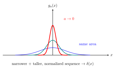
三维 Dirac delta 不是普通有限函数;其核心性质是
\[\int_{\mathbb R^3}\delta^{(3)}(\mathbf r-\mathbf r_0)\,d^3r=1,\]
\[\boxed{ \int f(\mathbf r)\delta^{(3)}(\mathbf r-\mathbf r_0)\,d^3r =f(\mathbf r_0) }.\]
\(\delta^{(3)}\) 的单位为 \(\mathrm{m^{-3}}\)。位于 \(\mathbf r_0\) 的点电荷 \(q\) 表示为
\[\boxed{\rho(\mathbf r)=q\delta^{(3)}(\mathbf r-\mathbf r_0)}.\]
4.2 The hidden source at \(r=0\)
对 \(r\ne0\),直接微分给出
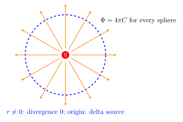
\[\nabla\cdot\left(\frac{\hat{\mathbf r}}{r^2}\right)=0.\]
但任意包围原点的球面通量是 \(4\pi\)。因此全空间正确的 distribution identity 是
\[\boxed{ \nabla\cdot\left(\frac{\hat{\mathbf r}}{r^2}\right) =4\pi\delta^{(3)}(\mathbf r) }.\]
点电荷场随即满足
\[\nabla\cdot\mathbf E =\frac{q}{4\pi\varepsilon_0}4\pi\delta^{(3)}(\mathbf r) =\frac{q\delta^{(3)}(\mathbf r)}{\varepsilon_0}.\]
4.3 Surface and line sources embedded in three dimensions
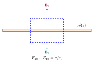
平面 \(z=0\) 上表面密度 \(\sigma(x,y)\) 可写
\[\rho(x,y,z)=\sigma(x,y)\delta(z).\]
\(z\) 轴上线密度 \(\lambda(z)\) 可写
\[\rho(x,y,z)=\lambda(z)\delta(x)\delta(y).\]
跨过表面的小 pillbox 对局部方程积分得到法向跳跃条件
\[\boxed{ \hat{\mathbf n}\cdot(\mathbf E_2-\mathbf E_1)=\frac{\sigma}{\varepsilon_0} }.\]
Worked Example 4 — Normalize a Gaussian point-charge model
以宽度 \(a\) 的光滑密度近似原点点电荷:
\[\rho_a(r)=\frac{q}{\pi^{3/2}a^3}e^{-r^2/a^2}.\]
- 系统与模型: 全空间球对称;\(a>0\) 时是普通函数,\(a\to0\) 时取 distribution 极限。
- 归一化:
\[\int\rho_a\,d^3r =\frac{4\pi q}{\pi^{3/2}a^3} \int_0^\infty r^2e^{-r^2/a^2}dr.\]
利用 \(\int_0^\infty r^2e^{-r^2/a^2}dr=\sqrt\pi a^3/4\),得到
\[\int\rho_a\,d^3r=q.\]
- 极限解释: 任意连续测试函数 \(f\) 有
\[\lim_{a\to0}\int f(\mathbf r)\rho_a(\mathbf r)d^3r=qf(0),\]
故 \(\rho_a\to q\delta^{(3)}(\mathbf r)\)。
- 检查: 前因子单位 \(q/a^3\) 为 \(\mathrm{C/m^3}\);总电荷对 \(a\) 不变,不是峰高本身守恒。
Lesson synthesis / 全课整合
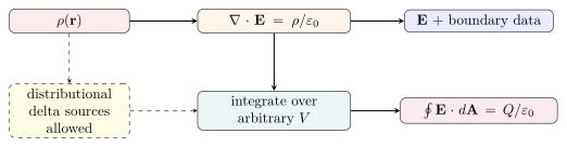
Formula-and-decision table
| Task | Equation | Conditions / boundary |
|---|---|---|
| compute divergence | \(\partial_xE_x+\partial_yE_y+\partial_zE_z\) | Cartesian components |
| coordinate-free meaning | \(\lim_{\Delta V\to0}\Delta V^{-1}\oint\mathbf E\cdot d\mathbf A\) | shrinking volume avoids singular point |
| infer smooth density | \(\rho=\varepsilon_0\nabla\cdot\mathbf E\) | also test curl for electrostatics |
| recover integral law | integrate over \(V\) + divergence theorem | piecewise smooth or distribution framework |
| point charge at \(\mathbf r_0\) | \(\rho=q\delta^{(3)}(\mathbf r-\mathbf r_0)\) | delta has unit \(\mathrm{m^{-3}}\) |
| charged interface | \(E_{2n}-E_{1n}=\sigma/\varepsilon_0\) | normal points from region 1 to 2 |
Model boundaries / 模型边界
- 宏观连续 \(\rho\) 是粗粒化模型;原子尺度需量子与微观物质理论。
- 点电荷是理想化 singular source;其经典自场与自能在 \(r=0\) 发散。
- 对不连续场,普通逐点导数可能漏掉 delta;须用积分或 distribution。
- \(\nabla\cdot\mathbf E=\rho/\varepsilon_0\) 不能单独唯一确定 \(\mathbf E\);还需 curl 与边界条件。
- 介质中若仍写总微观电荷,方程保持真空形式;宏观 \(\mathbf D\) 形式将在 Unit 4.4 另行定义。
Misconception clinic / 易错概念诊所
| Misconception | Correction |
|---|---|
| “散度大说明 \(E\) 大。” | 散度看局部净流出;均匀强场可很大而散度为零。 |
| “\(\rho=0\) 就有 \(\mathbf E=0\)。” | 只能得散度为零;远处源和边界仍可产生非零场。 |
| “等积分一次就能等被积函数。” | 必须对任意体积成立。 |
| “点电荷外散度为零,所以没有源。” | \(r=0\) 有 \(4\pi\delta^{(3)}\) 的隐藏贡献。 |
| “delta 在原点等于无穷就是定义。” | 严格定义是对测试函数的积分作用;“无限尖峰”仅是直觉。 |
| “满足 Gauss 局部式就一定是静电场。” | 还需 \(\nabla\times\mathbf E=0\) 与边界条件。 |
Practice and retrieval / 练习与检索
- 求 \(\mathbf E=(ax,by,cz)\) 的散度与对应 \(\rho\)。
Answer 1
\(\nabla\cdot\mathbf E=a+b+c\),\(\rho=\varepsilon_0(a+b+c)\)。
- \(\mathbf E=E_0\hat{\mathbf x}\) 的散度是多少?它能否在无电荷区非零?
Answer 2
散度为 0;能,均匀场可以由区域外的边界电荷建立。
- \(\mathbf E=ky\hat{\mathbf x}\) 的散度为什么为零?
Answer 3
\(E_x\) 不随 \(x\) 变,且其余分量为零,所以 \(\partial_xE_x=0\);\(\partial_yE_x\) 不进入散度。
- 从局部方程恢复半径 \(R\) 球内的积分 Gauss law。
Answer 4
对球体积分:\(\int_V\nabla\cdot\mathbf E\,dV=\varepsilon_0^{-1}\int_V\rho dV\);用散度定理左边变为 \(\oint_S\mathbf E\cdot d\mathbf A\)。
- 位于 \((a,0,0)\) 的点电荷 \(q\) 写成何种密度?
Answer 5
\(\rho=q\delta(x-a)\delta(y)\delta(z)=q\delta^{(3)}(\mathbf r-a\hat{\mathbf x})\)。
- 均匀线电荷沿 \(z\) 轴时写出三维密度并核对单位。
Answer 6
\(\rho=\lambda\delta(x)\delta(y)\);单位 \((\mathrm{C/m})(\mathrm{m^{-2}})=\mathrm{C/m^3}\)。
- 平面 \(z=z_0\) 上均匀面密度 \(\sigma\) 的三维表示是什么?
Answer 7
\(\rho=\sigma\delta(z-z_0)\),单位 \(\mathrm{C/m^2}\times\mathrm{m^{-1}}=\mathrm{C/m^3}\)。
- 真空界面两侧法向场为 \(E_{1n}=100\ \mathrm{N/C}\)、\(E_{2n}=400\ \mathrm{N/C}\),求 \(\sigma\)。
Answer 8
\(\sigma=\varepsilon_0(E_{2n}-E_{1n})=2.66\times10^{-9}\ \mathrm{C/m^2}\)。
- 为什么 \(\nabla\cdot(\hat{\mathbf r}/r^2)=0\) 的普通计算不与球面通量 \(4\pi\) 矛盾?
Answer 9
普通计算只适用于 \(r\ne0\);原点的 distribution 项 \(4\pi\delta^{(3)}(\mathbf r)\) 恰补回球面通量。
- 给出一个 \(\rho=0\) 但不是静电场的矢量场。
Answer 10
例如 \(\mathbf E=(-\omega y,\omega x,0)\):散度为零但 curl 为 \(2\omega\hat{\mathbf z}\),故不是静电场。
Exit ticket
用一条等式和一句边界说明解释:为什么点电荷场在每个 \(r>0\) 点都无散,却仍是原点电荷的正确场?
Exit-ticket benchmark
\(\nabla\cdot(\hat{\mathbf r}/r^2)=4\pi\delta^{(3)}(\mathbf r)\);普通零散度只适用于不含奇点的 \(r>0\) 区域,任何包围原点的体积积分仍得到 \(4\pi\)。
References and source notes / 参考资料与来源说明
以下直接来源均于 2026-08-26 实际访问核验。
- MIT OCW 6.641 — Maxwell's Differential Laws in Free Space
- MIT OCW 8.022 Lecture 3 — Gauss's Law Revisited and Divergence
- MIT OCW 6.007 Lecture 5 — Electrostatics: Gauss's Law and Boundary Conditions
- Richard Fitzpatrick, UT Austin — Electric Scalar Potential
- MIT OCW, Electromagnetic Fields and Energy, Chapter 2
Source-to-content map
| Source | Used for | Knowledge ID / Section | Model boundary or convention |
|---|---|---|---|
| MIT 6.641 Ch. 2 | divergence from incremental volume; arbitrary-volume logic | K01, K02 | distinguish theorem from physical law |
| MIT 8.022 Lecture 3 | undergraduate field/divergence cross-check | K01–K03 | Cartesian and integral forms |
| MIT 6.007 Lecture 5 | integral/differential Gauss law and electrostatic boundary conditions | K02, K03 | SI convention; pillbox/local-limit logic |
| Fitzpatrick UT Austin | \(\nabla\cdot\mathbf E=\rho/\varepsilon_0\) from Coulomb field | K02, K04 | singular origin handled distributionally |
| MIT EFE Chapter 2 | integral/differential Maxwell laws and charge conservation context | synthesis | local equation requires boundary information |
复习与拓展
- Electric Potential 将引入 \(\mathbf E=-\nabla V\),随后 Poisson 方程把 divergence 与 potential 合并。
- Unit 4.4 的介质界面会把法向跳跃推广到 \(\mathbf D\) 与自由电荷。
- 后续数值电磁学可把有限体积法视为本课“微盒通量平衡”的离散版本。