
Learning objectives / 学习目标
辨认 ferro/antiferro/ferrimagnetic sublattices;解释 domain formation 和 hysteresis 能量账本;区分 \(T_C\)、\(T_N\) 与外场下 crossover;比较 Ising/Heisenberg 自由度;使用 long-wavelength magnon dispersion 计算能量和 group velocity。
Prerequisites / 先修知识
- Microscopic Magnetic Moments 的 exchange sign convention。
- Free energy、entropy、order parameter、Fourier waves 与 harmonic approximation。
Scope and conventions / 范围与约定
- 使用 \(H=-J\sum_{\langle ij\rangle}\mathbf S_i\cdot\mathbf S_j\);\(J>0\) ferro。
- \(M\) 是 net magnetization;antiferromagnet 另用 staggered order \(L=M_A-M_B\)。
- 磁滞是路径依赖的非平衡响应;面积表示每体积每周期能量损耗,不能由 equilibrium equation of state 单独给出。
- 只讲 nearest-neighbor ideal models;frustration、dipolar textures 与 quantum spin liquids 作为边界。
Notation and modeling contract / 符号与建模契约
| Symbol | Meaning | SI unit |
|---|---|---|
| \(M_s\) | saturation magnetization | \(\mathrm{A\,m^{-1}}\) |
| \(H_c\) | coercive field | \(\mathrm{A\,m^{-1}}\) |
| \(T_C,T_N\) | Curie/Néel temperature | K |
| \(J\) | exchange energy scale | J |
| \(a\) | lattice spacing | m |
| \(\omega(k)\) | magnon angular frequency | \(\mathrm{s^{-1}}\) |
1. Ferromagnetism, antiferromagnetism, and ferrimagnetism / 铁磁、反铁磁与亚铁磁
Knowledge ID: P09-U05-L02-K01
有序方向还可能不是严格共线。Spin–orbit coupling 允许弱 canting,使名义 antiferromagnet 出现小净磁矩;螺旋或锥形结构则需要 ordering wavevector 与旋转平面共同描述。此时只使用“平行或反平行”会丢失关键信息。最小报告应包含 magnetic unit cell、各 sublattice moment、传播矢量和外场条件,才能把宏观磁化与 microscopic arrangement 一一对应。
不同有序还对应不同 symmetry breaking 与 reciprocal-space signatures。Ferromagnetic ordering vector 通常为 \(q=0\),antiferromagnetic pattern 则在非零 ordering vector 出现磁峰;ferrimagnet 同时具有 staggered component 与 uniform component。若 sublattice moments 随温度下降速率不同,net magnetization 甚至可在 compensation temperature 穿零而两子晶格仍保持有序。故“净磁化为零”既可能是 antiferromagnet,也可能是 ferrimagnet 的 compensation point,必须结合 microscopic pattern 判断。
判断磁有序不能只看总磁化。铁磁体在零场选取一个自发磁化方向,破坏自旋旋转或反演相关对称性;反铁磁体的两个子晶格磁矩等大反向,总磁矩虽为零,交错磁化却非零;亚铁磁体同样反向排列,但离子种类、占位或磁矩大小不同,因而留下净磁矩。实验上应结合中子衍射的磁布拉格峰、磁化曲线和温度依赖,而不能把“磁铁能吸铁”当成分类标准。外场还可能让反铁磁自旋发生倾斜或自旋翻转,所以有限场净磁矩并不自动改变零场有序类别。建模时必须声明子晶格、交换符号、easy axis 和被测 order parameter。
Ferromagnet 的 order parameter 是非零 net \(M\);antiferromagnet 的相邻 sublattices 反平行且等大,net \(M\) 可为零但 staggered \(L\ne0\);ferrimagnet 也反平行,却因两 sublattice moments 不等而保留 net \(M\)。判断必须看 ordering pattern,而非只测零场总磁矩。
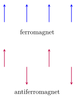
图 1 对比 net 与 staggered order。
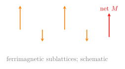
图 2 显示 unequal antiparallel moments 的非零合成。
2. Domains, walls, and hysteresis / 磁畴、畴壁与磁滞
Knowledge ID: P09-U05-L02-K02
Wall motion 的能垒产生 Barkhausen jumps,说明宏观平滑 loop 实际由许多离散重排平均而成。快速扫场时动态滞后与 eddy currents 还会扩大曲线面积,所以材料数据必须注明频率。微小颗粒若尺寸低于稳定 wall 的尺度,会转为 single-domain rotation;再减小后 thermal activation 可造成 superparamagnetic blocking,显示 domain 概念本身也有尺寸边界。
Soft magnet 追求低 coercivity 与小 loop loss,适合 transformer core;hard magnet 依靠强 anisotropy 与 pinning 保存 remanence,适合 permanent magnet。两者不是“exchange 强弱”的简单排序。Sample shape 改变 demagnetizing field,grain boundaries 和 precipitates 改变 wall pinning,temperature 又改变 anisotropy;同一种 chemical composition 经不同 processing 可得到完全不同 loop。分析曲线时还需区分 \(B\)–\(H\) 与 \(M\)–\(H\) loop,二者面积与单位的解释不能混用。
磁畴来自多项能量的折衷。单畴可让 exchange 与 anisotropy 达到低能,却会在样品外产生较大退磁场;切成多个方向不同的畴可降低 stray-field energy,但每一条畴壁都要支付 exchange twist 和 anisotropy deviation 的能量。畴壁具有有限宽度,其尺度由 exchange stiffness 与 anisotropy 的比值控制。外场作用时,低能过程常先是有利畴通过 wall motion 长大,随后才是磁矩连续旋转;defect pinning 使反向过程走不同路径。于是 remanence、coercivity 和 loop area 都依赖微结构、扫场速率与历史,并非只由 saturation magnetization 决定。
单畴虽降低 exchange energy,却可能产生大的 stray-field energy。分畴降低 magnetostatic energy,但增加 domain-wall energy;平衡尺度来自竞争。外场移动 walls、旋转 moments 并跨越 pinning barriers,撤场后路径不回原点,形成 remanence 与 coercivity。
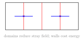
图 3 中红线是 finite-width wall 的简写,而非物理裂缝。
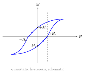
图 4 的 loop area 是 dissipated energy density \(\mu_0\oint H\,dM\);箭头标明路径。
3. Curie and Néel temperatures / 居里与奈尔温度
Knowledge ID: P09-U05-L02-K03
临界温度不是材料在所有条件下固定不变的孤立数字。Pressure、strain、composition 与 carrier density 都可改变 exchange paths,从而移动 transition。实验中 warming 与 cooling 若出现明显差异,可能提示 first-order character、结构耦合或 kinetic arrest,而理想连续相变模型并不包含这些历史效应。给出温度时还应说明测量 observable 与判据,例如峰值、拐点或外推零点。
临界行为可写 \(M\propto(T_C-T)^\beta\)、\(\chi\propto|T-T_C|^{-\gamma}\),但 exponents 取决于 universality class,而非所有磁体都等于 mean-field 值。实验拟合必须避开 finite-size rounding、field rounding 与非临界背景。反铁磁 susceptibility 在 \(T_N\) 附近常表现 cusp 而非简单 divergence,因为 uniform field 并不直接耦合 staggered order。Heat capacity、neutron scattering 与 susceptibility 的联合证据比单一曲线更可靠。
相变温度表示 exchange energy 与 thermal entropy 的竞争达到临界,而不是单个磁矩在该温度突然消失。铁磁体在零场下以净磁化为序参量,在 \(T_C\) 上方长期平均恢复对称;反铁磁体则以交错磁化为序参量,在 \(T_N\) 上方失序。临界附近 correlation length 增大,局域自旋仍可能保留短程关联,因此“paramagnetic phase”不等同于完全独立。Curie–Weiss 外推得到的 \(\Theta\) 可提示主导 exchange sign,却不必严格等于实际 transition temperature;低维、frustration 与 fluctuation 会使 mean-field 预测严重偏移。有限样品或有限外场还会把尖锐奇点圆滑化。
\(T_C\) 是 ferro/ferrimagnetic spontaneous-order transition temperature;\(T_N\) 是 antiferromagnetic staggered order 消失温度。Mean-field Curie–Weiss susceptibility 常写 \(\chi=C/(T-\Theta)\),但临界附近涨落使 mean-field exponent 不可靠。有限外场会圆滑化 ferro 的零场奇点。
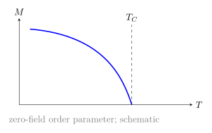
图 5 表示 \(T<T_C\) 的 spontaneous \(M\),不是外场诱导曲线。
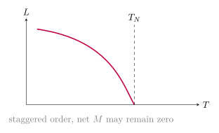
图 6 强调 antiferromagnet 的正确 order parameter 是 \(L\)。
4. Ising and Heisenberg spin models / 伊辛与海森堡自旋模型
Knowledge ID: P09-U05-L02-K04
边界条件会影响 finite lattice 的 apparent order:周期边界消除表面但限制允许 wavevectors,开放边界则产生 edge coordination reduction。比较理论与实验时应做 finite-size scaling,而不是把小系统平滑 crossover 当作 bulk critical point。Observable 也要对应模型自由度,例如 Ising magnetization 与 Heisenberg spin stiffness 回答的问题不同。
Quantum Ising model 再加入 transverse field 后,非对易项会在零温驱动 quantum phase transition;这与 classical thermal disorder 是不同机制。Heisenberg spins 的 operator components 也不同时可定,因此 classical arrows 只是 large-spin 或 mean-field 图像。数值模拟若把 quantum spin 换成 unit vectors,应明确这是 classical approximation;否则 transition temperature 与 excitation spectrum 的比较会混淆。
External field 在 Ising model 中直接偏置 \(s_i\),在 Heisenberg model 中还可引起连续 canting 和 spin-flop。加入 anisotropy term \(-K\sum(S_i^z)^2\) 可在两极限间插值;加入 competing next-neighbor exchange 则可能产生 frustration 与螺旋结构。Monte Carlo、mean field 与 spin-wave expansion 回答不同尺度的问题,使用结果时必须说明 thermodynamic limit、boundary condition 与 classical/quantum spin convention。
Ising 与 Heisenberg 的差别首先是自由度。强单轴晶体场把低能磁矩限制为沿 easy axis 的两个方向,适合离散 Ising variable;近各向同性磁体允许三维连续旋转,更接近 Heisenberg vector。两者即使使用同一个 nearest-neighbor \(J\),缺陷、domain wall、低能波和临界行为也不同。模型降维还必须考虑 spatial dimensionality:一维短程 Ising 在有限温度没有普通长程有序,二维连续对称模型的长波涨落受到 Mermin–Wagner 约束。真实材料的 weak anisotropy、long-range dipolar coupling 或 interlayer coupling 可以重新稳定有序,因此教材 lattice model 是受控近似,不是材料名称标签。
Ising variables \(s_i=\pm1\) 只能沿 easy axis,\(H=-J\sum s_is_j-h\sum s_i\);Heisenberg spins 可三维旋转,\(H=-J\sum\mathbf S_i\cdot\mathbf S_j\)。模型选择取决于 anisotropy 与 dimensionality,而不是计算方便。连续对称性会产生低能 Goldstone-like spin waves;二维短程 isotropic Heisenberg model 的有限温度有序受 Mermin–Wagner constraint。
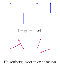
图 7 对比 configuration space。
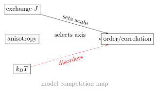
图 8 展示交换、各向异性与温度共同决定 correlation length。
5. Spin waves and magnons / 自旋波与磁振子
Knowledge ID: P09-U05-L02-K05
自旋波展开以 ordered ground state 为参考,把横向偏离当小量;靠近 transition 时 magnon density 大、相互作用强,线性理论不再受控。Ferromagnetic resonance 主要探测接近均匀 mode,中子散射可覆盖整个 Brillouin zone,两者给出的“gap”对应不同 wavevector。把低波数公式外推到 zone boundary 会违反 lattice periodicity,也会漏掉多支与 avoided crossings。
Magnon occupation obeys Bose statistics,但总 magnon number 通常不守恒;升温会增加 magnons 并降低 ordered moment。低温 ferro magnon 的 quadratic dispersion 导致特定 heat-capacity power law,antiferromagnetic linear modes 给另一幂律。若外场或 anisotropy 打开 gap,低温 population 会 exponential suppressed。Group velocity 控制能量传播,而 phase velocity 不等于单个 spin 的进动速度;谱线 linewidth 则记录 damping channels。
自旋波是有序背景上的协同小角度进动:相邻磁矩的相位缓慢改变,而各磁矩长度近似不变。量子化后,每个 normal mode 的一个能量量子称为 magnon,并携带明确 crystal momentum 与 spin angular momentum change。铁磁体因均匀旋转接近零能,常在低波数出现二次色散;反铁磁体两个子晶格耦合,常形成近线性色散。各向异性会在 \(k=0\) 打开 gap,有限温度的 magnon–magnon 与 magnon–phonon scattering 会产生 linewidth。中子散射测得的是 dynamical structure factor,因此从峰位置和宽度可分别读取 dispersion 与 lifetime,而非看见“一个翻转自旋移动”。
有序基态的小角度、长波长集体进动形成 spin wave;量子化后每个 mode 的 excitation 是 magnon。最近邻一维 ferro chain 的 linear spin-wave result 可写
\[\hbar\omega(k)=2JS[1-\cos(ka)]\simeq JS(ka)^2,\]
其中最后一步要求 \(ka\ll1\)。Antiferromagnet 常有线性低-\(k\) dispersion;anisotropy 可打开 gap。
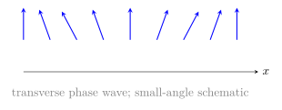
图 9 中每个 spin 的 cone phase 缓慢变化;它不是 particles 沿链移动。
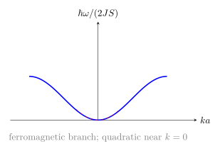
图 10 对照 lattice dispersion 与 long-wavelength approximation。
Worked Examples / 完整例题
Worked Example 1 — Ferrimagnetic net moment
完整建模协议: 下文把研究对象与系统边界限定在题目声明的样品或理想化子系统;参考系采用实验室静止系,并明确坐标正方向与所有矢量符号。模型选择必须由给定尺度和近似条件支持,不能只因公式方便。计算先写符号方程,再代入 SI 数值并保留适当有效数字;中间量与最终量均检查单位。求得结果后还要核对正负号、方向、量纲、极限情形和数量级,并解释它对应的可观测物理含义。若参数越出线性响应、长波长、弱场、高温或均匀介质等条件,则本例结论只能作为估算,必须换用更完整模型。
已知: sublattices \(M_A=4.0\times10^5\)、\(M_B=2.5\times10^5\ \mathrm{A\,m^{-1}}\),反平行。系统/轴: crystal volume,\(+z\) along A。模型: collinear two-sublattice。
\[M=M_A-M_B=1.5\times10^5\ \mathrm{A\,m^{-1}}.\]
检查: 小于任一 sum,方向 \(+z\)。解释: 非零 net moment 不等于 ferro coupling。
Worked Example 2 — Hysteresis loss
完整建模协议: 下文把研究对象与系统边界限定在题目声明的样品或理想化子系统;参考系采用实验室静止系,并明确坐标正方向与所有矢量符号。模型选择必须由给定尺度和近似条件支持,不能只因公式方便。计算先写符号方程,再代入 SI 数值并保留适当有效数字;中间量与最终量均检查单位。求得结果后还要核对正负号、方向、量纲、极限情形和数量级,并解释它对应的可观测物理含义。若参数越出线性响应、长波长、弱场、高温或均匀介质等条件,则本例结论只能作为估算,必须换用更完整模型。
已知: measured loop integral \(\oint H\,dM=1.8\times10^4\ \mathrm{A^2m^{-2}}\),频率 \(50\ \mathrm{Hz}\)。系统: unit volume core。模型: quasistatic SI loop。
\[w=\mu_0\oint H\,dM=2.26\times10^{-2}\ \mathrm{J\,m^{-3}},\quad P/V=fw=1.13\ \mathrm{W\,m^{-3}}.\]
检查: \(\mu_0HM\) 是 energy density。解释: eddy-current loss 未含在此磁滞面积模型中。
Worked Example 3 — Curie–Weiss estimate
完整建模协议: 下文把研究对象与系统边界限定在题目声明的样品或理想化子系统;参考系采用实验室静止系,并明确坐标正方向与所有矢量符号。模型选择必须由给定尺度和近似条件支持,不能只因公式方便。计算先写符号方程,再代入 SI 数值并保留适当有效数字;中间量与最终量均检查单位。求得结果后还要核对正负号、方向、量纲、极限情形和数量级,并解释它对应的可观测物理含义。若参数越出线性响应、长波长、弱场、高温或均匀介质等条件,则本例结论只能作为估算,必须换用更完整模型。
已知: \(C=0.80\ \mathrm K\),\(\Theta=300\ \mathrm K\),\(T=400\ \mathrm K\)。对象: paramagnetic phase。模型: mean field, \(T>\Theta\)。
\[\chi=C/(T-\Theta)=8.0\times10^{-3}.\]
检查: 无量纲;接近 \(\Theta\) 发散提示 mean-field/linear-response 失效。解释: 真正临界区要用 critical scaling。
Worked Example 4 — Magnon energy and velocity
完整建模协议: 下文把研究对象与系统边界限定在题目声明的样品或理想化子系统;参考系采用实验室静止系,并明确坐标正方向与所有矢量符号。模型选择必须由给定尺度和近似条件支持,不能只因公式方便。计算先写符号方程,再代入 SI 数值并保留适当有效数字;中间量与最终量均检查单位。求得结果后还要核对正负号、方向、量纲、极限情形和数量级,并解释它对应的可观测物理含义。若参数越出线性响应、长波长、弱场、高温或均匀介质等条件,则本例结论只能作为估算,必须换用更完整模型。
已知: \(JS=5.0\ \mathrm{meV}\),\(a=0.30\ \mathrm{nm}\),\(ka=0.20\)。系统: ferro chain,long wavelength。坐标: \(+x\) along chain。
\[E\simeq JS(ka)^2=0.200\ \mathrm{meV},\qquad v_g=\frac{1}{\hbar}\frac{dE}{dk}=\frac{2JSa(ka)}{\hbar}=9.12\times10^2\ \mathrm{m\,s^{-1}}.\]
检查: \(ka\ll1\);速度方向随 \(k\)。解释: damping 与 anisotropy 未计。
Lesson synthesis / 全课综合
Exchange 选择局域 alignment,lattice 与 anisotropy 选择 order parameter,自由能竞争决定 domains,pinning 造成 hysteresis,长波涨落量子化为 magnons。宏观曲线必须连接到合适的 equilibrium 或 nonequilibrium model。
Formula-and-decision table / 公式与决策表
| Task | Relation | Use when | Boundary |
|---|---|---|---|
| net ferrimagnetic \(M\) | \(M=M_A-M_B\) | collinear unequal sublattices | canting may add components |
| loop loss | \(w=\mu_0\oint H\,dM\) | closed quasistatic SI loop | excludes other losses |
| Curie–Weiss | \(\chi=C/(T-\Theta)\) | mean-field paramagnetic regime | critical fluctuations matter |
| Ising | \(H=-J\sum s_is_j\) | strong easy-axis anisotropy | discrete spins only |
| ferro magnon | \(E=2JS(1-\cos ka)\) | nearest-neighbor chain | convention/model dependent prefactor |
Model boundaries / 模型边界
- Domain size depends on geometry, demagnetization and defects.
- Hysteresis is rate- and history-dependent; no universal loop follows from \(J\) alone.
- \(T_C,T_N\) are thermodynamic limits; finite samples round transitions.
- Linear spin-wave theory assumes dilute magnons/small deviations from order.
Misconception clinic / 误区诊所
- Antiferromagnet net \(M=0\) does not mean no order.
- Ferrimagnet is not a weak ferromagnet; it has antiparallel unequal sublattices.
- Domain walls are finite-width spin textures, not material cracks.
- Coercivity is not the same as exchange strength.
- Magnon is a collective quantum, not one flipped spin traveling as a bead.
Practice and retrieval / 练习与提取
- [K01] Define staggered magnetization.
- [K01] Equal antiparallel sublattices classify as what order?
- [K02] Why can domains lower total energy?
- [K02] What does hysteresis-loop area represent?
- [K03] Distinguish \(T_C\) and \(T_N\).
- [K03] For \(C=1.2\ \mathrm K\), \(T-\Theta=200\ \mathrm K\), find \(\chi\).
- [K04] Which model suits a strong uniaxial magnet?
- [K04] Why does dimensionality matter for continuous symmetry?
- [K05] Expand \(1-\cos ka\) to leading order.
- [K05] If \(k\) doubles in quadratic regime, how do magnon energy and group velocity change?
Answers / 答案
- \(L=M_A-M_B\) or the alternating signed spin sum.
- Antiferromagnetic order.
- They reduce stray-field energy at the cost of wall energy.
- Dissipated energy density per cycle, \(\mu_0\oint H\,dM\).
- \(T_C\) ends ferro/ferrimagnetic net order; \(T_N\) ends antiferromagnetic staggered order.
- \(6.0\times10^{-3}\).
- Ising model as a first approximation.
- Long-wavelength fluctuations are stronger at low dimension and can destroy finite-\(T\) continuous-symmetry order.
- \(1-\cos ka\simeq(ka)^2/2\).
- Energy increases by 4; group velocity by 2.
Exit ticket / 离堂检验
- 画出 ferrimagnet 的两 sublattices 并标出 net \(M\)。
- 用 exchange–anisotropy–thermal fluctuation 三项解释为何材料在 \(T_C\) 附近改变 order。
References and source notes / 参考资料与来源说明
以下来源的链接与主题于 2026-08-30 核验;LSU 索引页通过官方索引复核,其余 MIT 资源直接打开核验:
- MIT OCW, Theory of Solids II, Local Moment Magnetism and Exchange. https://ocw.mit.edu/courses/8-512-theory-of-solids-ii-spring-2009/91a1068173b839057d8dfb97c8e6df02_MIT8_512s09_lec14_15.pdf
- MIT OCW, Electronic, Optical and Magnetic Properties of Materials, Lecture 24. https://ocw.mit.edu/courses/3-024-electronic-optical-and-magnetic-properties-of-materials-spring-2013/1e6cd7942a6e0514d806af7190d53538_MIT3_024S13_2012lec24.pdf
- LSU Physics, Statistical Mechanics 2023 lecture notes index (Heisenberg model, phase quantization, ferromagnetism). https://sauls.lsu.edu/teaching/7225/2023/notes.html
- MIT OCW 3.15, Magnetic Fundamentals. https://ocw.mit.edu/courses/3-15-electrical-optical-magnetic-materials-and-devices-fall-2006/resources/ho9_magnetic_fundamentals/
- MIT OCW 8.08, Ising Model. https://ocw.mit.edu/courses/8-08-statistical-physics-ii-spring-2005/resources/ising_model/
- MIT OCW 8.044, Final Problem 3, Spin Waves. https://ocw.mit.edu/courses/8-044-statistical-physics-i-spring-2013/27d79144664793039a264b1564296b8f_MIT8_044S13_Final.pdf
Source-to-content map
| Source | Used for | Knowledge ID / Section | Model boundary or convention |
|---|---|---|---|
| MIT 8.512 | exchange mechanisms | K01, K04 | simplified local-moment model |
| MIT 3.024 | ferro/antiferro/ferri and transition temperatures | K01, K03 | sign convention restated |
| LSU 7225 | Heisenberg, phase transitions, collective modes | K03–K05 | advanced derivations summarized |
| MIT 3.15 Magnetic Fundamentals | anisotropy, domains, domain walls, hysteresis, hard/soft magnets | K02 | quasistatic material response; geometry and pinning matter |
| MIT 8.08 Ising Model | discrete-spin order and phase transition | K03, K04 | equilibrium Ising idealization |
| MIT 8.044 Spin Waves | long-wavelength spin-wave and magnon calculation | K05 | harmonic/low-magnon-density limit |
复习与拓展
- 与 superconducting order 对照:两者都有 order parameter,但 gauge response 与 excitation spectrum 不同。
- 可扩展:domain-wall profile、critical exponents、spin stiffness、neutron scattering、frustration。