
Learning objectives / 学习目标
完成本课后,你应能:从角动量写出电子 orbital/spin moment 并判断符号;用能量与响应定义区分 dia/paramagnetism;从 spin-\(1/2\) 配分函数推导 Curie law 与 saturation;在明确 Hamiltonian convention 后计算 singlet–triplet exchange splitting;检查量纲、方向和模型边界。
Prerequisites / 先修知识
- Hydrogen Atom:\(\mathbf L,\mathbf S,\mathbf J\) 与 Zeeman splitting。
- Canonical partition function、Boltzmann factor、Pauli antisymmetry。
- \(\mathbf M\)、\(\mathbf H\)、\(\mathbf B\) 的 SI 区别;线性介质中 \(\mathbf M=\chi\mathbf H\)。
Scope and conventions / 范围与约定
- 电子电荷 \(q=-e\),其中 \(e>0\);电子 orbital moment 与 \(\mathbf L\) 反向。
- 采用 volume susceptibility,SI 中 \(\chi\) 无量纲。弱磁化时 \(B\simeq\mu_0H\) 仅用于简化 Curie 推导。
- Exchange 统一写 \(\hat H_{\rm ex}=-J\hat{\mathbf S}_1\cdot\hat{\mathbf S}_2\),故 \(J>0\) 偏好 parallel。采用 \(+J\) 的文献结论符号相反。
- Localized independent-moment Curie law 不适用于 Pauli metal、强场饱和、低温 exchange correlation 或 crystal-field singlet ground state。
Notation and modeling contract / 符号与建模契约
| Symbol | Meaning | SI unit |
|---|---|---|
| \(\boldsymbol\mu\) | magnetic moment | \(\mathrm{J\,T^{-1}}\) |
| \(\mu_B=e\hbar/(2m_e)\) | Bohr magneton | \(\mathrm{J\,T^{-1}}\) |
| \(g_s,g_J\) | spin/Landé factor | 1 |
| \(n\) | localized-moment density | \(\mathrm{m^{-3}}\) |
| \(\chi\) | volume susceptibility | 1 |
| \(J\) | exchange coefficient in stated convention | J divided by spin-product units |
1. Orbital and spin magnetic moments / 轨道与自旋磁矩
Knowledge ID: P09-U05-L01-K01
计算与实验之间还需一层约定:能级对外场的一阶斜率给磁矩投影,而不同方向的斜率可重建有效因子张量。若存在简并,必须先对微扰矩阵对角化,不能只取某个基底态的期望值。温度改变 excited crystal-field levels 的布居后,测得的有效磁矩也会变化。因此严谨报告应给出场方向、温区、拟合模型与量子化轴,并区分自由离子、局域离子和能带准粒子的符号。
从实验角度看,magnetic moment 是能量对外场的负导数,而不是只能靠“电流环”定义。Stern–Gerlach separation、Zeeman spectroscopy 和 magnetic resonance 分别探测投影、能级差与动态进动。多电子离子还要先用 Hund rules 确定 \(L,S,J\),再考虑晶场和 spin–orbit 的相对强弱。若轨道简并被完全解除,低能态可能只保留 effective spin;若简并部分保留,orbital contribution 与方向依赖不可忽略。报告磁矩时应说明是 saturation moment、effective Curie moment 还是 spectroscopic moment,因为三者在 correlated solid 中可能不同。
闭合 conventional current 的 magnetic moment 是 current times oriented area。电子带负电,电流方向与电子运动方向相反;量子化后得到
\[\hat{\boldsymbol\mu}_L=-\frac{e}{2m_e}\hat{\mathbf L} =-\frac{\mu_B}{\hbar}\hat{\mathbf L}, \qquad \hat{\boldsymbol\mu}_S=-g_s\frac{\mu_B}{\hbar}\hat{\mathbf S}.\]
这两个负号决定 Zeeman energy \(-\boldsymbol\mu\cdot\mathbf B\) 的排序。Spin 不是带电小球的经典自转;\(g_s\simeq2\) 是 relativistic quantum property。原子内 spin–orbit coupling 把 \(\mathbf L\) 与 \(\mathbf S\) 合成 \(\mathbf J\),常用 \(\boldsymbol\mu=-g_J\mu_B\mathbf J/\hbar\)。进入晶体后,crystal field 可 quench orbital degeneracy,effective \(g\) 甚至成为 tensor;自由离子 \(g_J\) 不能无条件搬用。
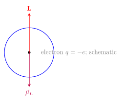
图 1 强调电子磁矩与 orbital angular momentum 反向;圆环是符号直觉,不是 stationary orbital 的经典轨迹。
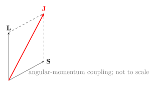
图 2 展示 vector-model coupling;真正允许的 \(J,m_J\) 仍由 quantum addition rules 给出。
2. Diamagnetic response / 抗磁响应
Knowledge ID: P09-U05-L01-K02
能量观点可写成外场下自由能的二阶曲率;负 susceptibility 表示系统通过诱导电流降低内部磁通变化。这个响应仍受边界条件约束:有限样品的测得磁化包含退磁场修正,各向异性晶体还需 susceptibility tensor。若测量采用 molar 单位,再与体积 susceptibility 比较时必须乘以摩尔体积。忽略这些换算会造成数量级正确却单位体系错误的假一致。
普通抗磁 susceptibility 往往很小,却几乎存在于所有电子体系。经典图像把外场视为改变 orbital angular frequency,而量子图像把 field-induced mixing 与 energy curvature 求和;两者都给出反向响应,但数值系数依赖 wavefunction 尺寸与能级结构。温度依赖通常弱,是因为 occupied closed-shell states 不靠 thermal population imbalance 工作。若样品同时含 paramagnetic impurities,总 susceptibility 是多种贡献之和,低温 \(1/T\) tail 甚至会掩盖 intrinsic diamagnetism;因此需做 background subtraction 与 concentration control,不能从一次正负号测量直接断言纯机制。
Diamagnetism 是外场改变 orbital motion 或 wavefunction 后产生的 induced response,方向反抗场,故 \(\chi<0\)。它不要求零场已有 permanent moment。Lenz-law 图景可判断方向,但定量 susceptibility 来自 minimal coupling 的 \(A^2\) 项与 occupied states 求和。Closed shells 的 permanent moments 相消,却仍可被场极化而抗磁。
抗磁体在 nonuniform field 中倾向低场区,因为 energy density 随 field 增大;均匀场不提供 center-of-mass force gradient。超导 Meissner response 也强烈抗磁,但来自 macroscopic phase stiffness 与 screening currents,不应当作 ordinary atomic diamagnetism 的放大版。
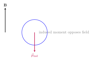
图 3 的反向 moment 表达 induced response,不声称电子轨道半径按图变化。
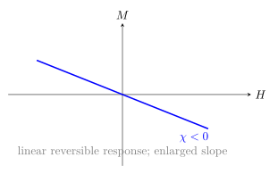
图 4 是 reversible line through origin,不是 ferromagnetic hysteresis loop。
3. Paramagnetism and Curie law / 顺磁性与居里定律
Knowledge ID: P09-U05-L01-K03
还应检查 demagnetizing correction:实验控制的是 applied field,而 moments 感受 local field。高磁化样品的形状会改变斜率,粉末平均又会抹平各向异性。只有先换算成一致的 internal-field convention,Curie constant 才能跨样品比较。
最后还要区分 isothermal 与 adiabatic susceptibility:若磁化过程快于热交换,spin temperature 会随场改变,响应不再等同于恒温导数。实际样品的晶格、核自旋和电子自旋具有不同 relaxation times,测量频率因此影响所得复 susceptibility。低频实部接近平衡斜率,虚部记录耗散与相位滞后。
对真实离子,磁矩大小常写成有效矩 \(g\sqrt{J(J+1)}\mu_B\),Curie constant 因而包含角动量简并信息。若低能只剩 Kramers doublet,可映射为 effective spin-\(1/2\),但各方向的 \(g\) 不同。实验拟合所得 effective moment 应与化学价态和晶场方案交叉检查;明显偏差可能来自 covalency、mixed valence 或短程关联,而不是简单的算术误差。
配分函数推导还揭示 entropy 的作用:零场时上下投影等概率、磁化为零但磁矩并未消失;加场降低平行能级后,population imbalance 产生净磁化。微分 susceptibility 是 \(\partial M/\partial H\),在非线性 regime 不再等于 \(M/H\)。若 moments 之间已有弱 exchange,常见经验形式变为 \(C/(T-\Theta)\);正负 \(\Theta\) 反映平均 correlation tendency,但 frustration 可让实际 ordering temperature 远低于 \(|\Theta|\)。因此用 Curie fit 时要展示 fitting window,并检验 field independence、impurity tail 与 saturation boundary。
Paramagnetism 来自可被 field bias 的 permanent moments。对 moment 投影 \(\pm\mu\),\(E_\pm=\mp\mu B\),单粒子 partition function 与 magnetization 为
\[Z_1=2\cosh\left(\frac{\mu B}{k_BT}\right), \qquad M=n\mu\tanh\left(\frac{\mu B}{k_BT}\right).\]
当 \(x=\mu B/(k_BT)\ll1\),\(\tanh x\simeq x\),于是
\[\chi=\frac{M}{H}\simeq\frac{\mu_0n\mu^2}{k_BT}=\frac{C}{T}.\]
Curie law 的 \(1/T\) 是 energy bias 与 thermal disorder 的竞争。低温或强场时 exact tanh curve saturation at \(M=n\mu\),线性外推会超过物理上限。一般 angular momentum \(J\) 使用 Brillouin function。Conduction-electron Pauli response 只涉及 Fermi surface 附近 states,低温通常近似与 \(T\) 无关。
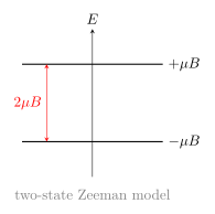
图 5 将 population imbalance 追溯到 Zeeman energy splitting。
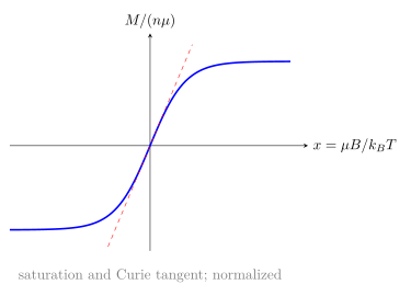
图 6 同时给出 weak-field tangent 与 saturation boundary。
4. Exchange interaction / 交换相互作用
Knowledge ID: P09-U05-L01-K04
若交换路径形成三角形或四面体,所有 pair preference 可能无法同时满足,产生 frustration。此时较大的 \(J\) 也未必带来高 ordering temperature,而可能保留大量低能 states。用 \(|\Theta|/T_N\) 的比例可初步衡量这种压低,但它仍是经验诊断。
数量级比较也很关键。两个 Bohr magnetons 相隔晶格常数的 dipolar energy 通常远低于典型 exchange energy;若实验 transition temperature 很高,单靠经典偶极作用难以解释。反之在稀磁体系或高度 frustrated material 中,较弱的 dipolar term 仍可能在最低温选择最终方向,因此“较小”不等于永远可删。
交换映射还要求能量分离:保留的 spin manifold 必须远低于被消去的 charge/orbital excitations。若 hopping 与 interaction 同量级,局域自旋长度本身会涨落,固定长度 Heisenberg model 失效。实验确定交换常数可用 susceptibility、specific heat、inelastic neutron scattering 或 resonance,但不同 observable 对多个 exchange paths 的组合敏感,因此需要结构对称性与全色散共同约束。
微观交换的最简来源可由 two-site Hubbard model 理解:electron hopping \(t\) 暂时产生 double occupancy,需付出 on-site repulsion \(U\),二阶过程给 antiferromagnetic scale \(J_{\rm AF}\sim4t^2/U\)。这说明交换能可远大于 classical dipole energy,也说明改变 bond angle、orbital occupancy 或 mediator atom 会改变 sign 和 magnitude。Direct exchange 强调 wavefunction overlap,superexchange 经非磁离子 virtual hopping,RKKY 经 conduction electrons 传播并可随距离振荡。映射到 Heisenberg model 前必须确认 charge fluctuations 已被冻结,否则单纯 localized-spin description 会漏掉 itinerant physics。
Exchange interaction 不是 classical dipole–dipole force。Identical-electron wavefunction 必须 antisymmetric;spatial symmetry 与 spin symmetry 绑定,而 Coulomb energy 对 spatial overlap 敏感。低能 subspace 中这些差异可压缩为
\[\hat H_{\rm ex}=-J\hat{\mathbf S}_1\cdot\hat{\mathbf S}_2.\]
由 \(\mathbf S_{\rm tot}^2=\mathbf S_1^2+\mathbf S_2^2+2\mathbf S_1\cdot\mathbf S_2\),两个 spin-\(1/2\) 的 triplet eigenvalue 是 \(\hbar^2/4\),singlet 是 \(-3\hbar^2/4\)。本课 convention 下 \(J>0\) lowers triplet;\(J<0\) lowers singlet。Direct exchange、superexchange、double exchange、RKKY 与 itinerant Stoner mechanisms 的 mediator 和 distance dependence 不同,不能仅凭“原子靠近”判断 sign。
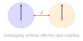
图 7 的彩色区域代表 wavefunction overlap,不是自旋之间的弹簧。
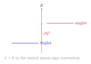
图 8 将 sign convention 直接编码到 level ordering。
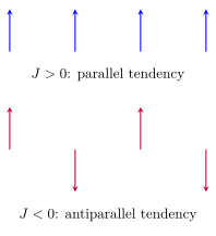
图 9 只表示 nearest-neighbor preference;finite temperature 与 frustration 可阻止 long-range order。

图 10 是诊断顺序:先确认 local degrees of freedom,再讨论 collective Hamiltonian。
Worked Examples / 完整例题
Worked Example 1 — Orbital projection and sign
完整建模协议: 下文把研究对象与系统边界限定在题目声明的样品或理想化子系统;参考系采用实验室静止系,并明确坐标正方向与所有矢量符号。模型选择必须由给定尺度和近似条件支持,不能只因公式方便。计算先写符号方程,再代入 SI 数值并保留适当有效数字;中间量与最终量均检查单位。求得结果后还要核对正负号、方向、量纲、极限情形和数量级,并解释它对应的可观测物理含义。若参数越出线性响应、长波长、弱场、高温或均匀介质等条件,则本例结论只能作为估算,必须换用更完整模型。
已知条件: electron state \(m_l=2\)。研究对象: isolated orbital moment。系统边界: 忽略 spin、crystal field 与 interactions。参考系/坐标: \(+z\) 为量子化轴。模型及理由: 使用 orbital moment operator,因为量子数已知。
\[\mu_{L,z}=-m_l\mu_B=-2(9.274\times10^{-24})=-1.85\times10^{-23}\ \mathrm{J\,T^{-1}}.\]
单位与有效数字: 三位有效数字,\(\mathrm{J\,T^{-1}}\)。方向检查: 负号表示 \(-z\)。极限检查: \(m_l=0\) 给零投影。物理解释: 结果是测量投影,不是 classical orbit vector length。
Worked Example 2 — Curie susceptibility
完整建模协议: 下文把研究对象与系统边界限定在题目声明的样品或理想化子系统;参考系采用实验室静止系,并明确坐标正方向与所有矢量符号。模型选择必须由给定尺度和近似条件支持,不能只因公式方便。计算先写符号方程,再代入 SI 数值并保留适当有效数字;中间量与最终量均检查单位。求得结果后还要核对正负号、方向、量纲、极限情形和数量级,并解释它对应的可观测物理含义。若参数越出线性响应、长波长、弱场、高温或均匀介质等条件,则本例结论只能作为估算,必须换用更完整模型。
已知条件: \(n=1.00\times10^{27}\ \mathrm{m^{-3}}\),\(\mu=\mu_B\),\(T=300\ \mathrm K\)。对象: independent localized moments。系统: unit material volume。坐标: field along \(+z\)。模型: weak-field Curie limit;需另检查 \(\mu B\ll k_BT\)。
\[\chi=\frac{\mu_0n\mu_B^2}{k_BT}=2.61\times10^{-5}.\]
单位检查: SI factors cancel,\(\chi\) 无量纲。方向: positive response。极限: \(T\to\infty\) 时趋零。解释: 若 moments itinerant,应改用 Pauli model。
Worked Example 3 — Strong-field saturation test
完整建模协议: 下文把研究对象与系统边界限定在题目声明的样品或理想化子系统;参考系采用实验室静止系,并明确坐标正方向与所有矢量符号。模型选择必须由给定尺度和近似条件支持,不能只因公式方便。计算先写符号方程,再代入 SI 数值并保留适当有效数字;中间量与最终量均检查单位。求得结果后还要核对正负号、方向、量纲、极限情形和数量级,并解释它对应的可观测物理含义。若参数越出线性响应、长波长、弱场、高温或均匀介质等条件,则本例结论只能作为估算,必须换用更完整模型。
已知条件: \(B=5.00\ \mathrm T\),\(T=2.00\ \mathrm K\),\(\mu=\mu_B\)。对象: spin-\(1/2\) ensemble。边界: independent two-state moments。坐标: \(+z\parallel\mathbf B\)。模型: exact tanh rather than Curie expansion。
\[x=\frac{\mu_BB}{k_BT}=1.68, \qquad \frac{M}{n\mu_B}=\tanh(1.68)=0.933.\]
检查: \(0<M/(n\mu_B)<1\)。Curie extrapolation gives \(1.68>1\) and is impossible。解释: exact partition function restores saturation。
Worked Example 4 — Singlet–triplet exchange splitting
完整建模协议: 下文把研究对象与系统边界限定在题目声明的样品或理想化子系统;参考系采用实验室静止系,并明确坐标正方向与所有矢量符号。模型选择必须由给定尺度和近似条件支持,不能只因公式方便。计算先写符号方程,再代入 SI 数值并保留适当有效数字;中间量与最终量均检查单位。求得结果后还要核对正负号、方向、量纲、极限情形和数量级,并解释它对应的可观测物理含义。若参数越出线性响应、长波长、弱场、高温或均匀介质等条件,则本例结论只能作为估算,必须换用更完整模型。
已知条件: two spin-\(1/2\),\(J\hbar^2=2.00\ \mathrm{meV}\) in \(H=-J\mathbf S_1\cdot\mathbf S_2\)。对象/系统: isolated two-spin manifold,无外场。坐标: total-spin basis。模型: isotropic Heisenberg exchange。
\[E_t=-\frac{J\hbar^2}{4}=-0.500\ \mathrm{meV}, \qquad E_s=\frac{3J\hbar^2}{4}=1.50\ \mathrm{meV},\]
\[E_s-E_t=2.00\ \mathrm{meV}.\]
检查: \(J>0\) 下 triplet lower,与 convention 相符。边界: anisotropy 或额外 orbitals 会 split triplet/modify mapping。解释: splitting 可通过 spectroscopy 或 thermodynamics 间接测量。
Lesson synthesis / 全课综合
微观磁性按“moment—response—correlation”组织:charge 与 angular momentum 决定单粒子 moment;field 对 occupied states 的重排产生 induced diamagnetism 或 population paramagnetism;exchange 再把不同 sites 关联。建模时先决定 localized/itinerant,再声明 \(H\) 或 \(B\) convention,最后验证 weak-field、high-temperature 与 low-energy projection 的条件。
Formula-and-decision table / 公式与决策表
| Task | Relation | Use only when | Boundary |
|---|---|---|---|
| orbital moment | \(\boldsymbol\mu_L=-\mu_B\mathbf L/\hbar\) | electron orbital angular momentum | crystal field can quench \(L\) |
| spin moment | \(\boldsymbol\mu_S=-g_s\mu_B\mathbf S/\hbar\) | effective spin specified | \(g\) may be anisotropic |
| Curie law | \(\chi=\mu_0n\mu^2/(k_BT)\) | independent, weak-field localized moments | not saturation or Pauli response |
| exact two-state \(M\) | \(M=n\mu\tanh(\mu B/k_BT)\) | two projections | larger \(J\) uses Brillouin function |
| exchange | \(H=-J\mathbf S_1\cdot\mathbf S_2\) | this note's convention | always state sign convention |
Model boundaries / 模型边界
- Classical loops provide sign intuition, not stationary-orbital trajectories。
- Volume, molar and mass susceptibilities differ by density factors。
- Curie law neglects exchange; Curie–Weiss behavior emerges when correlations matter。
- Isotropic pair exchange omits spin–orbit anisotropy, Dzyaloshinskii–Moriya coupling, itinerancy and frustration。
- Effective moments in solids depend on crystal-field level occupancy and temperature。
Misconception clinic / 误区诊所
- “Spin 是电子表面自转。” 内禀 angular momentum 不等于 extended charged sphere rotation。
- “Closed shell 没有磁响应。” Permanent moments 可相消,induced diamagnetism 仍存在。
- “所有 paramagnet 都有 \(1/T\)。” Pauli response 与 Van Vleck response 不遵从简单 Curie law。
- “交换是两个小磁铁的偶极力。” 其主因是 antisymmetry、Coulomb energy 与 virtual hopping。
- “\(J>0\) 的含义无需说明。” Hamiltonian 前的正负号决定标签。
Practice and retrieval / 练习与提取
- [K01 定义] 写出 Bohr magneton 及 SI 单位。
- [K01 方向] \(m_l=-1\) 时 \(\mu_{L,z}\) 的方向为何?
- [K02 图像] 线性抗磁体 \(M\)–\(H\) slope 的符号是什么?
- [K02 边界] 为什么均匀场通常不给小抗磁样品净平移力?
- [K03 推导] 从 \(\tanh x\simeq x\) 推出 \(\chi\propto1/T\)。
- [K03 判断] 温度翻倍时 ideal Curie susceptibility 如何变化?
- [K03 定量] \(n=2.00\times10^{26}\ \mathrm{m^{-3}}\)、\(\mu=2\mu_B\)、\(T=100\ \mathrm K\),求 \(\chi\)。
- [K04 概念] 本课 convention 下 \(J<0\) 偏好何种 two-spin state?
- [K04 推导] 求 singlet 的 \(\mathbf S_1\cdot\mathbf S_2\) eigenvalue。
- [综合] 金属 susceptibility 低温近似常数,应优先选择 Curie 还是 Pauli picture?
Answer 1
- \(\mu_B=e\hbar/(2m_e)=9.274\times10^{-24}\ \mathrm{J\,T^{-1}}\)。
Answer 2
2. \(\mu_{L,z}=-m_l\mu_B=+\mu_B\),沿 \(+z\)。
Answer 3
3. 负,因为 \(\chi<0\)。
Answer 4
4. 平移 dipole force 需要 field gradient;uniform field 不产生 center-of-mass energy gradient。
Answer 5
5. \(M=n\mu\tanh(\mu B/k_BT)\simeq n\mu^2B/(k_BT)\),结合 \(B\simeq\mu_0H\) 得 \(\chi\propto1/T\)。
Answer 6
6. 减为一半。
Answer 7
7. \(\chi=\mu_0n(2\mu_B)^2/(k_BT)=6.26\times10^{-5}\)。
Answer 8
8. Antiparallel/singlet tendency。
Answer 9
9. \(-3\hbar^2/4\)。
Answer 10
10. Pauli picture;degenerate conduction electrons 只有 Fermi surface 邻近 states 响应,故低温近似常数。
Exit ticket / 离堂检验
- 用同一张能量账本区分 induced diamagnetism、thermal paramagnetism 与 exchange correlation。
- 设计一个 temperature/field scan 判断某样品的 Curie law 在何处失效,并列出两种可能机制。
References and source notes / 参考资料与来源说明
以下直接来源于 2026-08-30 实际打开核验;正文重新组织,图示依据方程原创:
- MIT OCW, Theory of Solids II, Lectures 14–15: Local Moment Magnetism and Exchange Interactions. https://ocw.mit.edu/courses/8-512-theory-of-solids-ii-spring-2009/91a1068173b839057d8dfb97c8e6df02_MIT8_512s09_lec14_15.pdf
- MIT OCW, Introduction to Statistical Physics, Lecture 6. https://ocw.mit.edu/courses/res-8-010-introduction-to-statistical-physics-summer-2018/mitres_8_010su17_lec6.pdf
- MIT OCW, Electronic and Mechanical Properties of Materials, Lecture 12. https://ocw.mit.edu/courses/3-225-electronic-and-mechanical-properties-of-materials-fall-2007/resources/lecture_12/
- MIT OCW, Electronic, Optical and Magnetic Properties of Materials, Lecture 24. https://ocw.mit.edu/courses/3-024-electronic-optical-and-magnetic-properties-of-materials-spring-2013/1e6cd7942a6e0514d806af7190d53538_MIT3_024S13_2012lec24.pdf
Source-to-content map
| Source | Used for | Knowledge ID / Section | Model boundary or convention |
|---|---|---|---|
| MIT 8.512 | local moments, crystal field, exchange routes | K01, K04 | advanced mechanisms reduced to UG2 |
| MIT RES.8-010 | two-state partition function and Curie law | K03 | weak-field/high-\(T\) limit explicit |
| MIT 3.225 | filled shells and microscopic material response | K01, K02 | qualitative materials context |
| MIT 3.024 | exchange field and ordering tendency | K04 | sign convention restated in this note |
复习与拓展
- 下一课由 exchange、anisotropy 与 entropy 建立 ferro/antiferro/ferrimagnetic order。
- 与 magnetic resonance 相连:effective \(g\) tensor 与 local field 决定 resonance frequency。
- 可扩展:Landé derivation、Van Vleck response、Hubbard superexchange、RKKY、Dzyaloshinskii–Moriya coupling。