
Learning objectives / 学习目标
完成本课后,你应当能够:
- 严格区分平均速度、平均速率、瞬时速度和瞬时速率,尤其说明平均速率一般不等于平均速度的大小。
- 用速度变化定义平均与瞬时加速度,并用符号组合判断速度大小增减。
- 在 \(x\)–\(t\)、\(v\)–\(t\)、\(a\)–\(t\) 图之间使用斜率与有符号面积关系。
- 从常加速度定义推导运动方程,并在使用前验证时间区间内加速度确为常量。
- 在近地、常 \(g\)、忽略阻力的边界内处理自由落体,并说明失效尺度。
- 用微分从 \(x(t)\) 求 \(v(t),a(t)\),用定积分和初值从 \(a(t)\) 重建 \(v(t),x(t)\)。
0. Notation and sign discipline
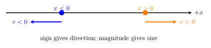
一维运动仍有方向。选定 \(+x\) 后,\(x,v,a\) 都可正、零或负;时间间隔满足 \(\Delta t>0\)。
| Quantity | Definition | SI unit |
|---|---|---|
| Position | \(x(t)\) | m |
| Displacement | \(\Delta x=x_f-x_i\) | m |
| Path length | \(s\ge0\) | m |
| Velocity | \(v=dx/dt\) | \(\mathrm{m/s}\) |
| Speed | \(u=\lvert v\rvert\) | \(\mathrm{m/s}\) |
| Acceleration | \(a=dv/dt\) | \(\mathrm{m/s^2}\) |
Knowledge 1 — Average and instantaneous speed and velocity / 平均与瞬时速率、速度
Knowledge ID: P01-U01-L02-K01
1.1 Interval quantities
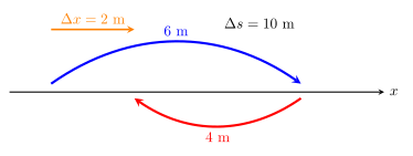
从 \(t_1\) 到 \(t_2\),\(\Delta t=t_2-t_1>0\):
\[\boxed{\overline v=\frac{\Delta x}{\Delta t}}\]
是平均速度,而
\[\boxed{\overline u=\frac{\Delta s}{\Delta t}}\]
是平均速率。因为 \(\Delta s\ge\lvert\Delta x\rvert\),所以
\[\boxed{\overline u\ge\lvert\overline v\rvert.}\]
只有区间内不反向时,两者才相等。平均速率不是“初、末速率的算术平均”;后者只在特定时间依赖下才成立。
1.2 Instantaneous limit and differentiability
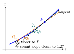
在时刻 \(t\),把区间缩小:
\[\boxed{ v(t)=\lim_{\Delta t\to0} \frac{x(t+\Delta t)-x(t)}{\Delta t} =\frac{dx}{dt} }.\]
瞬时速率为
\[\boxed{u(t)=\lvert v(t)\rvert.}\]
若 \(x(t)\) 在该时刻不可微,普通瞬时速度可能不存在。例如理想化的“瞬间反弹”在尖点处左右导数不同;真实碰撞需要有限作用时间的更精细模型。
1.3 Worked Example 1 — round trip average quantities
一名跑者从 \(x=0\) 出发,\(3.00\ \mathrm s\) 到 \(x=6.00\ \mathrm m\),再用 \(2.00\ \mathrm s\) 回到 \(x=2.00\ \mathrm m\)。
\[\Delta x=2.00\ \mathrm m, \qquad \Delta s=6.00+4.00=10.00\ \mathrm m, \qquad \Delta t=5.00\ \mathrm s.\]
因此
\[\overline v=+0.400\ \mathrm{m/s}, \qquad \overline u=2.00\ \mathrm{m/s}.\]
\(\overline u\ne\lvert\overline v\rvert\),差异正来自折返。两者单位相同,但定义中的分子不同。
Knowledge 2 — Average and instantaneous acceleration / 平均与瞬时加速度
Knowledge ID: P01-U01-L02-K02
2.1 Acceleration measures velocity change
区间平均加速度为
\[\boxed{\overline a=\frac{v_2-v_1}{t_2-t_1}=\frac{\Delta v}{\Delta t}.}\]
瞬时加速度是极限
\[\boxed{a(t)=\lim_{\Delta t\to0}\frac{\Delta v}{\Delta t}=\frac{dv}{dt}=\frac{d^2x}{dt^2}.}\]
加速度描述速度矢量的变化率,不等于“速度很大”,也不直接等于“越来越快”。
2.2 Four sign combinations
只要 \(v\ne0\):\(v\) 与 \(a\) 同号时速率增加,异号时速率减小。

在 \(v=0\) 的瞬间,不能只靠“同号/异号”规则判断之后运动;要看加速度和更高阶局部行为。抛到最高点的球有 \(v=0\)、\(a=-g\),并没有“加速度也为零”。
2.3 Worked Example 2 — negative acceleration is not always slowing down
给定
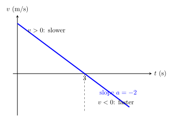
\[v(t)=6.00\ \mathrm{m/s}-(2.00\ \mathrm{m/s^2})t.\]
加速度恒为 \(a=-2.00\ \mathrm{m/s^2}\)。在 \(t=3.00\ \mathrm s\) 时 \(v=0\):
- \(0<t<3.00\ \mathrm s\):\(v>0,a<0\),速率减小;
- \(t>3.00\ \mathrm s\):\(v<0,a<0\),速率增加。
例如 \(t=4.00\ \mathrm s\) 时 \(v=-2.00\ \mathrm{m/s}\),物体沿负方向,速率为 \(2.00\ \mathrm{m/s}\) 并继续增加。
Knowledge 3 — Position-time, velocity-time, and acceleration-time graphs / 三类运动图像
Knowledge ID: P01-U01-L02-K03
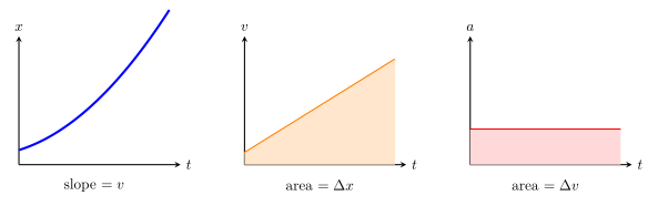
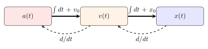
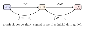
3.1 The derivative–integral ladder
\[\boxed{ x(t)\xrightarrow{\ d/dt\ }v(t)\xrightarrow{\ d/dt\ }a(t) }\]
反向用有符号面积并加初值:
\[\boxed{ \Delta v=\int_{t_1}^{t_2}a(t)\,dt, \qquad \Delta x=\int_{t_1}^{t_2}v(t)\,dt. }\]
所以:
- \(x\)–\(t\) 图切线斜率是 \(v\);
- \(v\)–\(t\) 图切线斜率是 \(a\);
- \(v\)–\(t\) 图与时间轴之间的有符号面积是位移,不一定是路程;
- \(a\)–\(t\) 图有符号面积是速度变化,不是速度本身。
3.2 Signed area versus total distance
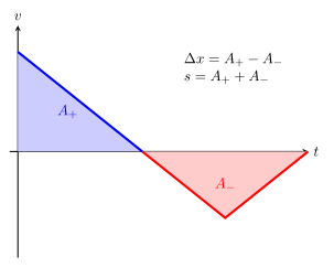
若 \(v\) 穿过零,净位移把时间轴上方与下方的面积相加(下方为负);路程则把每块面积取正后相加:
\[\Delta x=\int v\,dt, \qquad s=\int\lvert v\rvert\,dt.\]
3.3 Discontinuities and idealizations
位置在经典粒子模型中通常连续;位置若瞬间跳变意味着无限速度。速度可在理想化碰撞中画成跳跃,对应非常短时、很大的加速度脉冲,而不是普通有限函数。读图前要先问曲线代表真实分辨率还是极限模型。
Knowledge 4 — Constant-acceleration equations and their conditions / 匀变速公式及适用条件
Knowledge ID: P01-U01-L02-K04
4.1 Derivation, not formula collection
若在整个区间 \([t_0,t]\) 内 \(a\) 为常量,则积分 \(dv/dt=a\):
\[\boxed{v=v_0+a\Delta t}, \qquad \Delta t=t-t_0.\]
再积分 \(dx/dt=v_0+a(t-t_0)\):
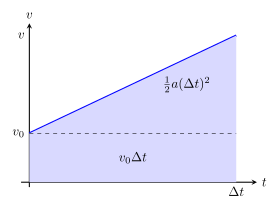
\[\boxed{x=x_0+v_0\Delta t+\frac12a(\Delta t)^2.}\]
由于 \(v\) 随时间线性变化,区间平均速度为
\[\overline v=\frac{v_0+v}{2},\]
故
\[\boxed{\Delta x=\frac{v_0+v}{2}\Delta t.}\]
消去 \(\Delta t\) 得
\[\boxed{v^2=v_0^2+2a\Delta x.}\]
4.2 Worked Example 3 — controlled braking
汽车沿 \(+x\) 方向以 \(v_0=24.0\ \mathrm{m/s}\) 开始制动,理想化为 \(a=-6.00\ \mathrm{m/s^2}\) 恒定,直到停止。
停止时间:
\[0=v_0+at_s \quad\Rightarrow\quad t_s=4.00\ \mathrm s.\]
制动位移:
\[\Delta x=v_0t_s+\frac12at_s^2 =24.0(4.00)-3.00(4.00)^2 =48.0\ \mathrm m.\]
用无时间式复核:
\[0-(24.0)^2=2(-6.00)\Delta x \quad\Rightarrow\quad \Delta x=48.0\ \mathrm m.\]
该结果只含制动阶段,不含驾驶员反应时间;若制动力随速率或路面变化,恒加速度模型也需替换。
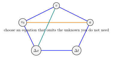
4.3 Choosing a relation by knowns, not by memory
Knowledge 5 — Free fall near a planet's surface / 近地自由落体
Knowledge ID: P01-U01-L02-K05
5.1 Local uniform-gravity model
自由落体指物体只受重力作用的理想运动;它不等同于“正在向下”。在地球表面附近、竖直尺度 \(h\ll R_E\) 且忽略空气阻力时,可取
\[\boxed{a_y=-g,\qquad g\approx9.81\ \mathrm{m/s^2}}\]
其中规定向上为 \(+y\)。于是
\[v_y=v_{0y}-gt,\]
\[y=y_0+v_{0y}t-\frac12gt^2.\]
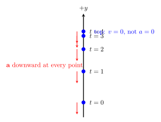
物体质量不出现在这些运动学方程中;在真空且同一初始条件下,不同质量物体具有相同 \(g\)。在空气中,阻力与形状、面积、速度和介质有关,运动一般不再是恒加速度。
5.2 Scale boundary for constant \(g\)
球形天体外部的重力加速度大小随中心距离近似按 \(1/r^2\) 变化。若从表面升高 \(h\),相对变化的一阶估计为
\[\frac{\lvert\Delta g\rvert}{g}\approx\frac{2h}{R}.\]
地球 \(R_E\approx6.37\times10^6\ \mathrm m\)。对 \(h=100\ \mathrm m\),变化约 \(3.1\times10^{-5}\),常 \(g\) 很好;对卫星轨道或行星际尺度必须改用位置依赖模型。
5.3 Worked Example 4 — upward throw from a platform
从离地 \(y_0=5.00\ \mathrm m\) 的平台竖直上抛小球,\(v_0=12.0\ \mathrm{m/s}\),忽略空气阻力,取 \(g=9.81\ \mathrm{m/s^2}\)。
最高点由 \(v=0\) 得
\[t_{\rm top}=\frac{v_0}{g}=1.223\ \mathrm s,\]
\[y_{\rm top}=y_0+\frac{v_0^2}{2g} =5.00+\frac{144}{19.62} =12.34\ \mathrm m.\]
落地时间解
\[0=5.00+12.0t-4.905t^2.\]
取物理上的正根:
\[t=\frac{12.0+\sqrt{(12.0)^2+2(9.81)(5.00)}}{9.81} =2.809\ \mathrm s.\]
落地速度
\[v=12.0-9.81(2.809)=-15.56\ \mathrm{m/s}.\]
负号表示向下;用 \(v^2=v_0^2+2(-g)(-5.00)\) 得速率 \(15.56\ \mathrm{m/s}\),与时间法一致。末位多保留一位用于两种方法的数值交叉检查;按输入的三位有效数字报告为 \(15.6\ \mathrm{m/s}\)。
Knowledge 6 — Kinematics from derivatives and integrals / 用微分与积分描述运动
Knowledge ID: P01-U01-L02-K06
6.1 State reconstruction needs initial conditions
导数会消去常数,因此从 \(a(t)\) 重建运动必须给初始条件。若在 \(t_0\) 有 \(v_0,x_0\):
\[\boxed{ v(t)=v_0+\int_{t_0}^{t}a(\tau)\,d\tau },\]
\[\boxed{ x(t)=x_0+\int_{t_0}^{t}v(\tau)\,d\tau }.\]
\(\tau\) 是积分中的哑变量,避免把上限 \(t\) 与积分变量混淆。
6.2 Worked Example 5 — variable acceleration
给定
\[a(t)=(3.00\ \mathrm{m/s^3})t-(2.00\ \mathrm{m/s^2}),\]
且 \(v(0)=4.00\ \mathrm{m/s}\)、\(x(0)=-1.00\ \mathrm m\)。积分得
\[v(t)=(4.00\ \mathrm{m/s}) +(1.50\ \mathrm{m/s^3})t^2 -(2.00\ \mathrm{m/s^2})t,\]
\[x(t)=(-1.00\ \mathrm m)+(4.00\ \mathrm{m/s})t -(1.00\ \mathrm{m/s^2})t^2 +(0.500\ \mathrm{m/s^3})t^3.\]
在 \(t=2.00\ \mathrm s\):
\[a=4.00\ \mathrm{m/s^2}, \qquad v=6.00\ \mathrm{m/s}, \qquad x=7.00\ \mathrm m.\]
单位检查:\(t^2\) 项系数必须是 \(\mathrm{m/s^3}\) 才能得到速度;\(t^3\) 项系数必须是 \(\mathrm{m/s^3}\) 才能得到位置。将 \(x(t)\) 连续求两次导数可恢复原 \(a(t)\)。
6.3 Nonsmooth motion and piecewise calculus
若运动在某时刻改变规则,应分段定义并检查边界处位置是否连续、速度是否连续。例如交通灯处突然改用另一恒加速度段,不能把两段不同 \(a\) 当作一个全区间常量。积分仍适用,但必须按分段边界拆开。
7. Lesson synthesis / 全课整合
7.1 One chain, two directions
7.2 Diagnostic workflow
- 选轴并画出正方向。
- 写已知量的带符号值,不把速率直接当速度。
- 判断所问是区间平均量还是瞬时量。
- 检查 \(a\) 是否在整个区间恒定;若否,用导数/积分或分段模型。
- 图像题先标斜率或有符号面积,再运算。
- 求路程时找出 \(v=0\) 的转向点并分段取绝对值。
- 检查单位、初值、极限、符号与数量级。
7.3 Approximation map
| Model | Reliable when | Main failure signal |
|---|---|---|
| Instantaneous derivative | \(x(t)\) 在该时刻可微 | 尖点、跳跃或测量噪声尺度过细 |
| Constant acceleration | 全区间 \(a\) 可视为常量 | \(a(t)\)、\(a(x)\) 或阻力明显变化 |
| Local constant \(g\) | \(h/R\ll1\) 且所需精度较低 | 轨道尺度、长距离落体或精密测量 |
| Vacuum free fall | 阻力和浮力远小于重力效应 | 终端速度、形状依赖或强风 |
| Smooth graph area | 曲线代表的连续模型有效 | 碰撞脉冲、离散采样不足 |
8. Misconception clinic / 易错概念诊所
| Misconception / 错误观念 | Correction / 修正 |
|---|---|
| “平均速率就是平均速度的大小。” | 折返时 \(\overline u>\lvert\overline v\rvert\);前者用路程,后者用位移。 |
| “瞬时量就是取一段极短但有限的平均。” | 严格定义是区间趋零的极限;实验只能用有限差分近似。 |
| “加速度为负就是减速。” | 要比较 \(v\) 与 \(a\) 的符号;同号速率增、异号速率减。 |
| “速度为零时加速度也为零。” | 上抛最高点 \(v=0\) 而 \(a=-g\)。 |
| “\(v\)–\(t\) 图下面的面积总是路程。” | 有符号面积是位移;路程需积分 \(\lvert v\rvert\)。 |
| “\(a\)–\(t\) 面积是速度。” | 它是 \(\Delta v\),还要加初速度。 |
| “匀变速公式可用平均加速度代替任意变加速。” | 一般不行;平均加速度只保证端点速度变化,不能恢复位移历史。 |
| “自由落体一定向下运动。” | 上抛后的上升段也属于自由落体,只是速度向上、加速度向下。 |
| “重物在真空中一定落得更快。” | 同地同初值、忽略非重力效应时 \(g\) 与测试物质量无关。 |
| “积分后不需要初值。” | 每次积分都会引入常数;初始状态决定具体轨迹。 |
9. Practice and retrieval / 练习与检索
A. Conceptual questions
- 一个往返过程什么时候有 \(\overline u=\lvert\overline v\rvert\)?
- \(v<0,a>0\) 时速率怎样变化?物体向哪边运动?
- \(x\)–\(t\) 图水平、向下倾斜、凹向上分别说明什么?
- 为什么 \(v^2=v_0^2+2a\Delta x\) 不能保留速度方向的全部信息?
- 上抛最高点附近,\(v\) 和 \(a\) 分别是什么?
- 从 \(a(t)\) 积分一次为什么不能唯一得到 \(v(t)\)?
B. Quantitative and derivation questions
- 物体 \(4.0\ \mathrm s\) 内从 \(x=-2.0\ \mathrm m\) 到 \(x=10.0\ \mathrm m\),途中路程 \(20.0\ \mathrm m\)。求平均速度与平均速率。
- \(v(t)=5.0-3.0t\)(SI)。求 \(t=1.0\ \mathrm s\) 的速度、速率、加速度,并判断当时速率变化。
- \(v\)–\(t\) 图在 \(0\le t\le4.0\ \mathrm s\) 为从 \(v=2.0\) 线性升到 \(v=10.0\ \mathrm{m/s}\)。求加速度和位移。
- 列车以 \(30.0\ \mathrm{m/s}\) 行驶,以 \(-1.50\ \mathrm{m/s^2}\) 恒加速度制动。求停止时间和位移。
- 从静止释放物体,自由落下 \(20.0\ \mathrm m\),忽略阻力,取 \(g=9.81\ \mathrm{m/s^2}\)。求时间和落地速率。
- 给定 \(a(t)=(4.0\ \mathrm{m/s^3})t\)、\(v(0)=-2.0\ \mathrm{m/s}\)、\(x(0)=1.0\ \mathrm m\)。求 \(v(t),x(t)\) 与 \(t=2.0\ \mathrm s\) 的状态。
- 证明对任意一维可微运动,只要区间内不反向,就有 \(s=\lvert\Delta x\rvert\)。
Answers / 参考答案
1. 区间内不反向(允许短暂停止但不改变运动方向)时。
2. 物体沿负方向,\(v\) 与 \(a\) 异号,速率减小。
3. 水平表示静止;向下倾斜表示 \(v<0\);凹向上表示 \(a>0\)(可微处)。
4. 平方消去 \(v\) 的正负号,必须结合运动阶段与方向判断。
5. 瞬时 \(v=0\),但 \(a=-g\)。
6. 积分产生常数,需给一个时刻的速度。
7. \(\overline v=12.0/4.0=3.00\ \mathrm{m/s}\);\(\overline u=20.0/4.0=5.00\ \mathrm{m/s}\)。
8. \(v=2.0\ \mathrm{m/s}\),\(u=2.0\ \mathrm{m/s}\),\(a=-3.0\ \mathrm{m/s^2}\);异号,速率减小。
9. \(a=(10.0-2.0)/4.0=2.00\ \mathrm{m/s^2}\);梯形面积 \(\Delta x=(2.0+10.0)4.0/2=24.0\ \mathrm m\)。
10. \(t_s=20.0\ \mathrm s\);\(\Delta x=300\ \mathrm m\)。
11.
\[t=\sqrt{\frac{2h}{g}}=2.02\ \mathrm s,
\qquad
u=gt=19.8\ \mathrm{m/s}.\]
12.
\[v(t)=(-2.0\ \mathrm{m/s})+(2.0\ \mathrm{m/s^3})t^2,\]
\[x(t)=(1.0\ \mathrm m)-(2.0\ \mathrm{m/s})t
+(0.667\ \mathrm{m/s^3})t^3.\]
在 \(t=2.0\ \mathrm s\),\(a=8.0\ \mathrm{m/s^2}\)、\(v=6.0\ \mathrm{m/s}\)、\(x=2.33\ \mathrm m\)。
13. 不反向意味着 \(v\) 在除静止点外保持同号,所以 \(s=\int\lvert v\rvert dt=\lvert\int vdt\rvert=\lvert\Delta x\rvert\)。
Exit ticket
不查公式,画出一条“先向 \(+x\) 加速、再减速到停、随后向 \(-x\) 加速”的 \(v\)–\(t\) 草图,并标出哪些区间 \(v,a\) 同号、哪些异号,以及怎样从图求净位移和路程。
10. References and source notes / 参考资料与使用说明
10.1 Source-to-content map
| Source | Used for |
|---|---|
| OpenStax, University Physics Volume 1, §3.1 Position, Displacement, and Average Velocity | interval definitions, signed displacement, distance traveled and position–time representation |
| OpenStax, §3.2 Instantaneous Velocity and Speed | limit definition, tangent interpretation, instantaneous speed |
| OpenStax, §3.3 Average and Instantaneous Acceleration | acceleration definitions and sign analysis |
| OpenStax, §3.4 Motion with Constant Acceleration | constant-acceleration derivations and graph areas |
| OpenStax, §3.5 Free Fall | local constant-\(g\) model and upward/downward cases |
| OpenStax, §3.6 Finding Velocity and Displacement from Acceleration | integration with initial conditions and variable acceleration |
| NASA Glenn, Falling Object with Air Resistance | explicit contrast between vacuum constant-\(g\) motion and drag-limited fall |
| MIT OpenCourseWare 8.01SC, Classical Mechanics | undergraduate kinematics sequencing and modeling boundaries |
10.2 Bibliographic notes
OpenStax §§3.1–3.6 form the main derivation spine. NASA Glenn is used only to audit the no-drag boundary. MIT 8.01SC provides an independent undergraduate course-level cross-check.