
Learning objectives / 学习目标
完成本课后,你应当能够:
- 对平行且匀速平移的经典惯性系写出 Galilean 位置、时间、速度和加速度变换,并说明低速边界。
- 使用对象—参照物下标法构造一维和多维相对速度闭合链,避免凭语言猜加减号。
- 从极坐标基矢的时间导数推导完整的 \(\mathbf v\) 与 \(\mathbf a\),解释四个加速度项。
- 推导旋转基底的 transport theorem,并由此得到一般平移—转动参考系中的速度、加速度关系。
- 区分纯运动学变换项与真实相互作用;不把坐标产生的项提前当成新的物理力。
- 用静止、纯平移、纯转动、固定于转盘等极限检查公式。
0. Notation: object first, reference second
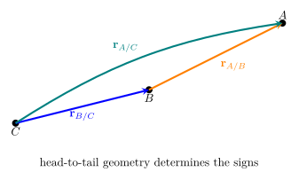
用
\[\mathbf r_{A/B}\]
表示“\(A\) 相对 \(B\) 的位置”,速度和加速度同理。两个基本规则是
\[\mathbf r_{A/B}=-\mathbf r_{B/A},\]
\[\boxed{ \mathbf r_{A/C}=\mathbf r_{A/B}+\mathbf r_{B/C} }.\]
中间下标 \(B\) 像单位一样首尾相消。对同一时间变量求导,就得到速度与加速度闭合链。
Knowledge 1 — Galilean transformation of position and velocity / 位置与速度的伽利略变换
Knowledge ID: P01-U01-L04-K01
1.1 Translating parallel frames
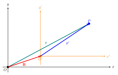
设 \(S\) 的原点为 \(O\),\(S'\) 的原点 \(O'\) 在 \(S\) 中的位置为 \(\mathbf R(t)\),两套轴始终平行。对事件/粒子 \(P\):
\[\boxed{ \mathbf r_{P/O}=\mathbf R(t)+\mathbf r_{P/O'} }.\]
简写为
\[\boxed{\mathbf r'=\mathbf r-\mathbf R(t).}\]
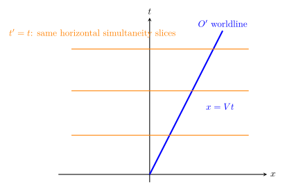
经典 Galilean 变换还假设所有地点共享绝对时间,最多差一个固定的时钟零点:
\[t'=t-t_*,\]
通常选 \(t_*=0\)。若 \(O'\) 以恒速度 \(\mathbf V\) 移动,且在 \(t=0\) 两原点重合,\(\mathbf R=\mathbf Vt\):
\[\boxed{ \mathbf r'=\mathbf r-\mathbf Vt, \qquad t'=t }.\]
求导得
\[\boxed{\mathbf v'=\mathbf v-\mathbf V,}\]
\[\boxed{\mathbf a'=\mathbf a}\]
其中最后一式要求 \(\mathbf V\) 恒定。若平移原点加速,\(\mathbf A=d\mathbf V/dt\),则
\[\mathbf a'=\mathbf a-\mathbf A.\]
1.2 Spacetime picture of simultaneity in the Galilean model
1.3 Worked Example 1 — event and velocity in a train frame
列车相对地面沿 \(+x\) 以 \(V=20.0\ \mathrm{m/s}\) 匀速运动,\(t=0\) 时两原点重合。地面系中,乘客在 \(t=5.00\ \mathrm s\) 位于 \(x=115\ \mathrm m\),并以 \(v=21.5\ \mathrm{m/s}\) 沿 \(+x\) 运动。
\[x'=x-Vt=115-20.0(5.00)=15.0\ \mathrm m,\]
\[v'=v-V=1.50\ \mathrm{m/s}.\]
乘客相对列车向前走 \(1.50\ \mathrm{m/s}\);相对地面速度更大。若他相对列车保持恒速,则两系测得的加速度均为零。
Knowledge 2 — Relative velocity in one and multiple dimensions / 一维与多维相对速度
Knowledge ID: P01-U01-L04-K02
2.1 The subtraction formula and chain rule
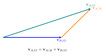
相对于公共参考物 \(O\):
\[\boxed{ \mathbf v_{A/B}=\mathbf v_{A/O}-\mathbf v_{B/O} }.\]
等价的闭合写法为
\[\boxed{ \mathbf v_{A/C} =\mathbf v_{A/B}+\mathbf v_{B/C} }.\]
不要根据“顺水加、逆水减”背符号;先写对象/参照物下标,再首尾相接。
2.2 One-dimensional closing and separation rates
两物体沿同一直线:
\[v_{A/B}=v_A-v_B.\]
若两者间有符号分离 \(x_{A/B}=x_A-x_B\),则
\[\frac{dx_{A/B}}{dt}=v_{A/B}.\]
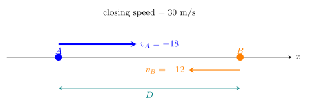
“closing speed / 接近速率”是距离减小率的正值,常写 \(-d\lvert x_{A/B}\rvert/dt\);它不是自动等于两个速率之和,符号取决于方向。
2.3 Worked Example 2 — two approaching trains
两列车相距 \(D=7.50\ \mathrm{km}\),且初始时 A 位于 B 的西侧。取东为正,A 向东 \(v_A=+20.0\ \mathrm{m/s}\),B 向西 \(v_B=-15.0\ \mathrm{m/s}\)。
\[v_{A/B}=20.0-(-15.0)=+35.0\ \mathrm{m/s}.\]
从 B 看,A 向东接近;距离以 \(35.0\ \mathrm{m/s}\) 减小。若速度保持不变:
\[t=\frac{7500\ \mathrm m}{35.0\ \mathrm{m/s}}=214\ \mathrm s=3.57\ \mathrm{min}.\]
若两列车同向,则接近速率变成速率之差;这说明用带符号速度统一处理最安全。
2.4 Worked Example 3 — boat across a river
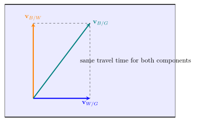
河宽 \(180\ \mathrm m\),水相对岸以 \(3.00\ \mathrm{m/s}\) 向东。船相对水以 \(4.00\ \mathrm{m/s}\) 正北航行。
\[\mathbf v_{B/G} =\mathbf v_{B/W}+\mathbf v_{W/G} =(3.00\widehat{\mathbf x}+4.00\widehat{\mathbf y})\ \mathrm{m/s}.\]
\[\lvert\mathbf v_{B/G}\rvert=5.00\ \mathrm{m/s}, \qquad \theta=\tan^{-1}(3/4)=36.9^\circ\]
即地面观察为北偏东 \(36.9^\circ\)。过河时间由北向分量决定:
\[t=180/4.00=45.0\ \mathrm s,\]
下游漂移
\[\Delta x=(3.00)(45.0)=135\ \mathrm m.\]
若要正对岸到达,船相对水需有 \(3.00\ \mathrm{m/s}\) 向西分量,剩余北向分量
\[v_N=\sqrt{4.00^2-3.00^2}=2.65\ \mathrm{m/s},\]
过河时间变为 \(68.0\ \mathrm s\)。
Knowledge 3 — Polar-coordinate velocity and acceleration / 极坐标中的速度与加速度
Knowledge ID: P01-U01-L04-K03
3.1 Polar geometry and moving unit vectors
平面极坐标用 \(r(t),\theta(t)\):
\[\mathbf r=r\widehat{\mathbf e}_r.\]
\[\widehat{\mathbf e}_r =\cos\theta\widehat{\mathbf x}+\sin\theta\widehat{\mathbf y},\]
\[\widehat{\mathbf e}_\theta =-\sin\theta\widehat{\mathbf x}+\cos\theta\widehat{\mathbf y}.\]
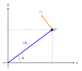
即使 \(r\) 不变,基矢也因 \(\theta\) 变化:
\[\boxed{ \dot{\widehat{\mathbf e}}_r =\dot\theta\widehat{\mathbf e}_\theta, \qquad \dot{\widehat{\mathbf e}}_\theta =-\dot\theta\widehat{\mathbf e}_r }.\]
3.2 Full velocity and acceleration derivation
对 \(\mathbf r=r\widehat{\mathbf e}_r\) 使用乘法法则:
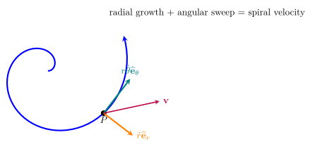
\[\boxed{ \mathbf v =\dot r\widehat{\mathbf e}_r +r\dot\theta\widehat{\mathbf e}_\theta }.\]
再次求导并合并同类项:
\[\boxed{ \mathbf a =(\ddot r-r\dot\theta^2)\widehat{\mathbf e}_r +(r\ddot\theta+2\dot r\dot\theta)\widehat{\mathbf e}_\theta }.\]
四个贡献为:
| Term | Kinematic origin | Direction |
|---|---|---|
| \(\ddot r\) | 径向速率变化 | \(\widehat{\mathbf e}_r\) |
| \(-r\dot\theta^2\) | 径向基矢转动 | \(-\widehat{\mathbf e}_r\) |
| \(r\ddot\theta\) | 角速度变化 | \(\widehat{\mathbf e}_\theta\) |
| \(2\dot r\dot\theta\) | 径向运动与基底转动的交叉项 | \(\widehat{\mathbf e}_\theta\) |
3.3 Worked Example 4 — expanding spiral
给定
\[r(t)=1.00\ \mathrm m+(0.200\ \mathrm{m/s})t, \qquad \theta(t)=(0.500\ \mathrm{rad/s^2})t^2.\]
在 \(t=2.00\ \mathrm s\):
\[r=1.40\ \mathrm m, \quad \dot r=0.200\ \mathrm{m/s}, \quad \ddot r=0,\]
\[\dot\theta=2.00\ \mathrm{rad/s}, \qquad \ddot\theta=1.00\ \mathrm{rad/s^2}.\]
速度分量:
\[v_r=0.200\ \mathrm{m/s}, \qquad v_\theta=r\dot\theta=2.80\ \mathrm{m/s},\]
\[v=\sqrt{0.200^2+2.80^2}=2.81\ \mathrm{m/s}.\]
加速度分量:
\[a_r=0-1.40(2.00)^2=-5.60\ \mathrm{m/s^2},\]
\[a_\theta=1.40(1.00)+2(0.200)(2.00)=2.20\ \mathrm{m/s^2},\]
\[a=\sqrt{(-5.60)^2+(2.20)^2}=6.02\ \mathrm{m/s^2}.\]
漏掉 \(2\dot r\dot\theta\) 会把 \(a_\theta\) 错算成 \(1.40\ \mathrm{m/s^2}\)。
3.4 Fast special-case checks
- 纯径向:\(\dot\theta=0\Rightarrow\mathbf v=\dot r\widehat{\mathbf e}_r\),\(\mathbf a=\ddot r\widehat{\mathbf e}_r\)。
- 匀速圆周:\(r=R\)、\(\dot\theta=\omega\) 常量,\(\mathbf a=-R\omega^2\widehat{\mathbf e}_r\)。
- 固定半径但变角速:再加 \(R\ddot\theta\widehat{\mathbf e}_\theta\)。
Knowledge 4 — Moving bases and rotating coordinates / 运动基底与旋转坐标
Knowledge ID: P01-U01-L04-K04
4.1 Transport theorem
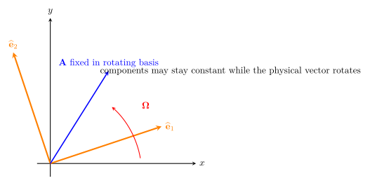
向量 \(\mathbf A\) 在旋转基底写成
\[\mathbf A=A_1\widehat{\mathbf e}_1+A_2\widehat{\mathbf e}_2+A_3\widehat{\mathbf e}_3.\]
基底以角速度 \(\boldsymbol\Omega\) 转动时
\[\left(\frac{d\widehat{\mathbf e}_i}{dt}\right)_I =\boldsymbol\Omega\times\widehat{\mathbf e}_i.\]
因此
\[\boxed{ \left(\frac{d\mathbf A}{dt}\right)_I =\left(\frac{d\mathbf A}{dt}\right)_R +\boldsymbol\Omega\times\mathbf A }.\]
左边是固定/惯性基底观察到的真实矢量变化率;右边第一项只微分旋转坐标中的分量,第二项补偿基底自身转动。
4.2 General velocity relation
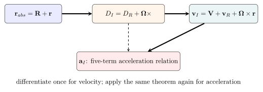
设旋转系原点 \(O'\) 相对惯性系 \(O\) 的位置为 \(\mathbf R(t)\),粒子相对 \(O'\) 的位置为 \(\mathbf r\)。绝对位置
\[\mathbf r_{P/O}=\mathbf R+\mathbf r.\]
用 transport theorem:
\[\boxed{ \mathbf v_I =\mathbf V_{O'} +\mathbf v_R +\boldsymbol\Omega\times\mathbf r }.\]
三项分别为原点平移、粒子相对旋转系的运动、基底转动携带速度。
4.3 General acceleration relation
再次对速度求惯性导数,并对 \(\mathbf v_R\) 使用 transport theorem:
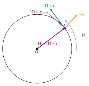
\[\boxed{ \begin{aligned} \mathbf a_I={}&\mathbf A_{O'}+\mathbf a_R +2\boldsymbol\Omega\times\mathbf v_R\\ &+\dot{\boldsymbol\Omega}\times\mathbf r +\boldsymbol\Omega\times(\boldsymbol\Omega\times\mathbf r). \end{aligned} }\]
| Term | Name / interpretation |
|---|---|
| \(\mathbf A_{O'}\) | rotating origin's translational acceleration |
| \(\mathbf a_R\) | acceleration measured from changing rotating-frame components |
| \(2\boldsymbol\Omega\times\mathbf v_R\) | Coriolis kinematic term |
| \(\dot{\boldsymbol\Omega}\times\mathbf r\) | Euler kinematic term |
| \(\boldsymbol\Omega\times(\boldsymbol\Omega\times\mathbf r)\) | inward centripetal transport term for a fixed rotating point |
4.4 Worked Example 5 — walking outward on a turntable
水平转盘以恒角速度
\[\boldsymbol\Omega=(1.50\ \mathrm{rad/s})\widehat{\mathbf z}\]
转动。某人相对转盘沿径向向外以 \(\mathbf v_R=0.500\widehat{\mathbf e}_r\ \mathrm{m/s}\) 匀速行走;某刻 \(r=2.00\ \mathrm m\)。取转盘中心固定,\(\dot{\boldsymbol\Omega}=0\),且在旋转坐标中径向速率恒定,所以 \(\mathbf a_R=0\)。
惯性系速度:
\[\mathbf v_I =0.500\widehat{\mathbf e}_r +(1.50)(2.00)\widehat{\mathbf e}_\theta =(0.500\widehat{\mathbf e}_r+3.00\widehat{\mathbf e}_\theta)\ \mathrm{m/s}.\]
加速度:
\[2\boldsymbol\Omega\times\mathbf v_R =1.50\widehat{\mathbf e}_\theta\ \mathrm{m/s^2},\]
\[\boldsymbol\Omega\times(\boldsymbol\Omega\times\mathbf r) =-\Omega^2r\widehat{\mathbf e}_r =-4.50\widehat{\mathbf e}_r\ \mathrm{m/s^2}.\]
因此
\[\mathbf a_I =(-4.50\widehat{\mathbf e}_r+1.50\widehat{\mathbf e}_\theta)\ \mathrm{m/s^2}, \qquad a_I=4.74\ \mathrm{m/s^2}.\]
这与极坐标式一致:\(\dot r=0.500\)、\(\dot\theta=1.50\)、\(\ddot r=\ddot\theta=0\),故 \(a_r=-r\dot\theta^2=-4.50\),\(a_\theta=2\dot r\dot\theta=1.50\)。
4.5 A derivation map worth memorizing
5. Lesson synthesis / 全课整合
5.1 Nested hierarchy
- Parallel, fixed offset: \(\mathbf r'=\mathbf r-\mathbf b\)。
- Parallel, translating origin: \(\mathbf r'=\mathbf r-\mathbf R(t)\)。
- Constant-velocity Galilean frames: \(\mathbf v'=\mathbf v-\mathbf V\),\(\mathbf a'=\mathbf a\)。
- Polar moving basis: \(\widehat{\mathbf e}_r,\widehat{\mathbf e}_\theta\) rotate with \(\dot\theta\)。
- General rotating frame: use \(D_I=D_R+\boldsymbol\Omega\times\) and retain all transport terms.
5.2 Diagnostic workflow
- 明确对象和参照物,下标按“对象/参照物”书写。
- 先画位置或速度头尾相接图,再写闭合等式。
- 判断两套轴是平行平移还是相对转动。
- 平行匀速系用 Galilean 变换;加速平移需保留原点加速度。
- 极坐标中每次求导都同时微分分量和基矢。
- 旋转系用 transport theorem,不靠死背五项。
- 用 \(\Omega=0\)、\(\mathbf v_R=0\)、\(r=\mathrm{constant}\) 等极限复核。
5.3 Approximation and boundary map
| Model | Reliable when | Main failure signal |
|---|---|---|
| Galilean transform | \(v\ll c\)、经典共同时间 | 相对论速度或高精度同步 |
| Acceleration invariance | 两系相对速度恒定且轴不转 | 原点加速或轴转动 |
| Simple velocity subtraction | 量均相对同一公共参考物 | 下标次序不闭合或混用参照系 |
| Polar formulas | 平面、\(r,\theta\) 光滑且基矢约定一致 | 在 \(r=0\) 角坐标奇异 |
| Rotating-frame relation | 刚性正交基底以单一 \(\boldsymbol\Omega\) 转动 | 变形基底需更一般张量方法 |
6. Misconception clinic / 易错概念诊所
| Misconception / 错误观念 | Correction / 修正 |
|---|---|
| “所有观察者测得同一速度。” | Galilean 系间速度相差参考系速度;恒速系只对加速度一致。 |
| “相对速度就是两个速率相加。” | 必须作矢量差 \(\mathbf v_{A/B}=\mathbf v_A-\mathbf v_B\)。 |
| “二维河流题可先把两个速率相加。” | 方向不同,必须矢量相加;过河时间由横河分量决定。 |
| “下标顺序不重要。” | \(\mathbf v_{A/B}=-\mathbf v_{B/A}\);次序决定方向。 |
| “极坐标只需把 \(x,y\) 换成 \(r,\theta\)。” | 极坐标基矢随时间转动,求导必须包含基矢导数。 |
| “\(a_\theta=r\ddot\theta\)。” | 当 \(\dot r\ne0\) 时还需 \(2\dot r\dot\theta\)。 |
| “离心项在惯性系加速度中向外。” | \(\boldsymbol\Omega\times(\boldsymbol\Omega\times\mathbf r)\) 对平面转动指向内;向外的“离心力”来自改写非惯性系动力学。 |
| “Coriolis 项表示一种新相互作用。” | 它是旋转基底下的运动学变换项,不由独立物体或场产生。 |
| “若物体固定在旋转坐标中,它的速度为零。” | 只是在该坐标中 \(\mathbf v_R=0\);惯性系仍有 \(\boldsymbol\Omega\times\mathbf r\)。 |
| “transport theorem 只适用于位置。” | 它适用于任意在旋转基底展开的矢量。 |
7. Practice and retrieval / 练习与检索
A. Conceptual questions
- 为什么两个匀速平移惯性系测得的加速度相同,而速度不同?
- 写相对速度链时,怎样用下标顺序检查等式?
- 船头正对彼岸为何通常不能正对岸到达?
- 在极坐标中,\(r\) 恒定是否意味着速度为零?
- \(2\dot r\dot\theta\) 项在什么条件下消失?
- 为什么固定在转盘上的点在转盘系 \(\mathbf a_R=0\),惯性系却有加速度?
- transport theorem 中哪一项来自基矢变化?
B. Quantitative and derivation questions
- \(S'\) 以 \(+8.0\ \mathrm{m/s}\) 相对 \(S\) 运动。粒子在 \(S\) 中 \(x=50\ \mathrm m\)、\(v=12.0\ \mathrm{m/s}\),时刻 \(t=4.0\ \mathrm s\),两原点初始重合。求 \(x',v'\)。
- A 向东 \(25\ \mathrm{m/s}\),B 向东 \(18\ \mathrm{m/s}\)。求 \(\mathbf v_{A/B}\) 与 \(\mathbf v_{B/A}\)。
- 飞机相对空气正北 \(200\ \mathrm{km/h}\),风相对地面正东 \(60\ \mathrm{km/h}\)。求地速大小和方向。
- 极坐标运动 \(r=2.0\ \mathrm m\)、\(\theta=0.50t^2\)(rad)。求 \(t=2.0\ \mathrm s\) 的 \(\mathbf v,\mathbf a\) 极坐标分量。
- 粒子满足 \(r=0.30t\ \mathrm m\)、\(\theta=2.0t\)(rad)。求 \(t=3.0\ \mathrm s\) 的速度和加速度分量。
- 转盘以 \(\Omega=2.0\ \mathrm{rad/s}\) 匀速转动。一个点固定在 \(r=0.50\ \mathrm m\)。用一般旋转系公式求惯性系速度和加速度。
- 从 transport theorem 连续使用两次,推导五项加速度关系,并标出系数 2 的来源。
Answers / 参考答案
1. 恒定平移速度在一次求导后留下常量差,在第二次求导时消失。
2. 右边相邻的中间参照物下标要相同,外侧下标组成左边。
3. 水流提供沿岸速度分量,地面轨迹是船相对水与水相对岸速度的矢量和。
4. 不意味着;若 \(\dot\theta\ne0\),\(\mathbf v=r\dot\theta\widehat{\mathbf e}_\theta\)。
5. \(\dot r=0\) 或 \(\dot\theta=0\)。
6. 固定分量并不等于固定物理矢量;基底转动产生 \(\boldsymbol\Omega\times(\boldsymbol\Omega\times\mathbf r)\)。
7. \(\boldsymbol\Omega\times\mathbf A\)。
8. \(x'=50-8.0(4.0)=18\ \mathrm m\);\(v'=12.0-8.0=4.0\ \mathrm{m/s}\)。
9. \(\mathbf v_{A/B}=+7.0\ \mathrm{m/s}\) 向东;\(\mathbf v_{B/A}=-7.0\ \mathrm{m/s}\),即向西。
10. \(v_G=\sqrt{200^2+60^2}=209\ \mathrm{km/h}\),北偏东 \(\tan^{-1}(60/200)=16.7^\circ\)。
11. \(\dot r=0\)、\(\dot\theta=t=2.0\ \mathrm{rad/s}\)、\(\ddot\theta=1.0\ \mathrm{rad/s^2}\):\(\mathbf v=4.0\widehat{\mathbf e}_\theta\ \mathrm{m/s}\);\(\mathbf a=(-8.0\widehat{\mathbf e}_r+2.0\widehat{\mathbf e}_\theta)\ \mathrm{m/s^2}\)。
12. 在 \(t=3.0\ \mathrm s\),\(r=0.90\ \mathrm m\):\(v_r=0.30\)、\(v_\theta=1.80\ \mathrm{m/s}\);\(a_r=-3.60\)、\(a_\theta=1.20\ \mathrm{m/s^2}\)。
13. \(\mathbf v=1.0\widehat{\mathbf e}_\theta\ \mathrm{m/s}\);\(\mathbf a=-2.0\widehat{\mathbf e}_r\ \mathrm{m/s^2}\)。
14. 对 \(\mathbf v_R\) 求导产生一项 \(\boldsymbol\Omega\times\mathbf v_R\);对 \(\boldsymbol\Omega\times\mathbf r\) 求导时又产生一项,合为 \(2\boldsymbol\Omega\times\mathbf v_R\)。
Exit ticket
从 \(\mathbf r_{abs}=\mathbf R+\mathbf r\) 出发,不查笔记写出一般旋转系速度式;然后用一句话说明为什么 \(\mathbf v_R=0\) 仍不能推出 \(\mathbf v_I=0\)。
8. References and source notes / 参考资料与使用说明
8.1 Source-to-content map
| Source | Used for |
|---|---|
| OpenStax, University Physics Volume 1, §4.5 Relative Motion in One and Two Dimensions | object/reference notation, one- and two-dimensional velocity addition, boat/wind structure, low-speed caveat |
| MIT OpenCourseWare 8.01SC, Online Textbook | classical reference frames and Chapter 31 non-inertial-frame route |
| MIT OpenCourseWare 8.01SC, Chapter 31 — Non-Inertial Rotating Reference Frames | rotating-basis derivative and interpretation of coordinate-generated terms |
| MIT OpenCourseWare 2.003SC, Velocity, Acceleration, and Rotational Motion | polar velocity/acceleration and translating/rotating coordinate systems |
| MIT OpenCourseWare 16.07, Lecture L7 — Relative Motion using Translating Axes | translating-frame position, velocity and acceleration relations |
| MIT OpenCourseWare 16.07, Lecture L8 — Relative Motion using Rotating Axes | transport theorem and full rotating-frame velocity/acceleration relations |
8.2 Bibliographic notes
OpenStax supplies the introductory relative-motion spine. MIT 2.003SC and 16.07 supply the UG1→UG2 moving-basis derivations. MIT 8.01SC is used to keep coordinate terms conceptually separate from real interactions and to connect forward to dynamics without doing it prematurely.