
Learning objectives / 学习目标
完成本课后,你应当能够:
- 从 \(K=E-U\ge0\) 确定一维保守运动的可达域、禁阻域、速率和普通转折点。
- 用扰动响应与势能局部形状区分稳定、不稳定和中性平衡,并知道 \(U''=0\) 时二阶判据不充分。
- 在非退化势阱极小值附近作 Taylor 展开,推导 \(\omega=\sqrt{U''(x_0)/m}\) 并判断小振幅近似范围。
- 将中心力径向运动改写成含角动量势垒的有效势问题,识别圆轨道、径向稳定性和可达半径。
- 明确势能图法要求能量守恒、一维或可约化自由度,并辨认耗散、显含时间势和多自由度耦合的边界。
0. Read dynamics from geometry

势能图不是“地形的实际高度图”。横轴是广义位置坐标,纵轴是能量;小球在山谷中滚动只是帮助理解 \(F=-dU/dx\) 的类比。
Knowledge 1 — Turning points and accessible regions / 转折点与可达区域
Knowledge ID: P01-U03-L04-K01
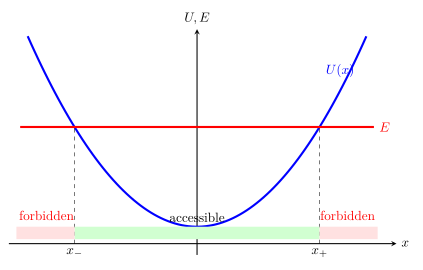
1.1 Allowed condition and speed branches
对一维保守系统,
\[E=K+U(x)=\frac12m\dot x^2+U(x).\]
由于经典动能非负,
\[\boxed{E-U(x)\ge0.}\]
因此:
- \(U(x)<E\):经典可达域,速率非零;
- \(U(x)>E\):经典禁阻域;
- \(U(x_t)=E\):\(\dot x=0\) 的候选转折点或平衡/分离轨道端点。
速率为
\[\boxed{\lvert\dot x\rvert=\sqrt{\frac{2[E-U(x)]}{m}},}\]
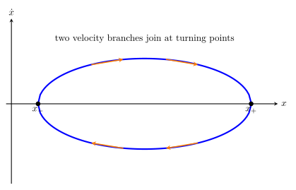
而速度有两支:
\[\dot x=\pm\sqrt{\frac{2[E-U(x)]}{m}}.\]
能量图本身不给出此刻选择哪一支;需由初始运动方向决定。
1.2 Ordinary turning points and separatrix caveat
若 \(U(x_t)=E\) 且 \(U'(x_t)\ne0\),则 \(F(x_t)=-U'(x_t)\ne0\),质点通常在有限时间到达、瞬时静止并反向,这是普通转折点。
若同时 \(U'(x_t)=0\),该点是平衡点。特别在能量恰等于局部最大值时,轨迹可作为分离轨道在无限长时间内渐近接近不稳定平衡,而不一定像普通转折点那样弹回。仅凭 \(E=U\) 不能跳过斜率检查。
1.3 Worked Example 1 — a double-well landscape
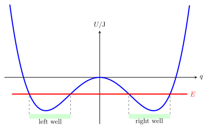
定义无量纲坐标 \(q=x/(1.00\ \mathrm m)\),势能为
\[U(x)=(2.00\ \mathrm J)(q^4-q^2).\]
给定总能量 \(E=-0.250\ \mathrm J\)。转折点满足
\[2(q^4-q^2)=-0.250,\]
\[q^4-q^2+0.125=0.\]
令 \(z=q^2\),
\[z=\frac{1\pm\sqrt{1-0.500}}{2} =0.1464\ \text{or}\ 0.8536.\]
所以
\[q=\pm0.3827,\quad\pm0.9239.\]
可达域为两个互不连通的势阱:
\[-0.9239\le q\le-0.3827,\]
\[0.3827\le q\le0.9239.\]
能量为负,质点无法穿过中央 \(U(0)=0\) 的势垒,因此初始在哪个阱就留在哪个阱。
Knowledge 2 — Stable, unstable, and neutral equilibrium / 稳定、不稳定与随遇平衡
Knowledge ID: P01-U03-L04-K02
2.1 Equilibrium condition and perturbation test
平衡点 \(x_0\) 满足
\[F(x_0)=-U'(x_0)=0.\]
分类关注小扰动后的行为:
- **Stable / 稳定:**足够小扰动后仍留在平衡附近;孤立严格极小值通常稳定。
- **Unstable / 不稳定:**任意小扰动可使系统离开;局部极大值通常不稳定。
- **Neutral / 中性或随遇:**沿某方向位移后仍处于新平衡,典型为势能在一段或一个流形上恒定。

2.2 Second-derivative test and degenerate cases
在 \(U'(x_0)=0\) 处:
\[U''(x_0)>0\Rightarrow\text{nondegenerate local minimum, stable},\]
\[U''(x_0)<0\Rightarrow\text{local maximum, unstable}.\]
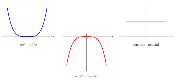
若 \(U''(x_0)=0\),二阶判据没有结论。例如 \(U=ax^4\)(\(a>0\))在 \(0\) 有稳定极小值,\(U=-ax^4\) 在 \(0\) 不稳定,而 \(U=\) constant 在整个区间中性。必须检查首个非零高阶项或直接用扰动定义。
2.3 Worked Example 2 — equilibria of the double well
仍用
\[U=(2.00\ \mathrm J)(q^4-q^2), \qquad q=\frac{x}{1.00\ \mathrm m}.\]
平衡条件 \(dU/dx=0\) 等价于
\[4q^3-2q=2q(2q^2-1)=0,\]
所以
\[q=0, \qquad q=\pm\frac{1}{\sqrt2}=\pm0.7071.\]
二阶导数为
\[\frac{d^2U}{dx^2} =\frac{2.00\ \mathrm J}{(1.00\ \mathrm m)^2}(12q^2-2).\]
在 \(q=0\),\(U''=-4.00\ \mathrm{J/m^2}<0\),不稳定;在 \(q=\pm1/\sqrt2\),\(U''=8.00\ \mathrm{J/m^2}>0\),稳定。两个极小值均为 \(U=-0.500\ \mathrm J\)。
2.4 Local versus global stability
局部极小值只保证小扰动被困在附近。如果能量输入超过相邻势垒,系统仍可逃离该势阱。稳定性必须连同扰动大小、允许的耗散/驱动和分析时间尺度说明。
Knowledge 3 — Small oscillations near a potential minimum / 势能极小值附近的小振动
Knowledge ID: P01-U03-L04-K03
3.1 Taylor expansion and harmonic reduction
令 \(x_0\) 为非退化稳定平衡:
\[U'(x_0)=0, \qquad \kappa\equiv U''(x_0)>0.\]
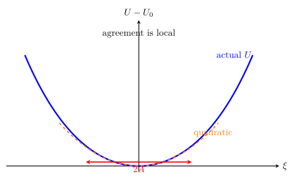
记小位移 \(\xi=x-x_0\)。Taylor 展开:
\[U(x_0+\xi) =U(x_0)+\frac12\kappa\xi^2 +\frac16U'''(x_0)\xi^3+\cdots.\]
在振幅足够小时保留二次项:
\[F=-\frac{dU}{dx}\approx-\kappa\xi.\]
运动方程成为
\[m\ddot\xi+\kappa\xi=0,\]
\[\boxed{\omega=\sqrt{\frac{U''(x_0)}{m}}, \qquad T=2\pi\sqrt{\frac{m}{U''(x_0)}}.}\]
3.2 Approximation criterion
若三次项是首个修正,一个实用条件是在 \(\lvert\xi\rvert\le A\) 内
\[\frac{\lvert U'''(x_0)\rvert A}{3U''(x_0)}\ll1\]
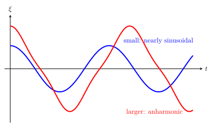
使三次势能项远小于二次项。若对称性令 \(U'''(x_0)=0\),需比较四次项。随着振幅增大,周期可能依振幅,波形也不再是纯正弦。
3.3 Worked Example 3 — frequency from curvature
在某稳定平衡 \(x_0\) 附近,
\[U(x)=U_0+(8.00\ \mathrm{J/m^2})(x-x_0)^2+\text{higher terms}.\]
与 \(U_0+\tfrac12\kappa(x-x_0)^2\) 比较:
\[\kappa=16.0\ \mathrm{N/m}.\]
若 \(m=2.00\ \mathrm{kg}\),则
\[\omega=\sqrt{\frac{16.0}{2.00}} =2.83\ \mathrm{rad/s},\]
\[T=\frac{2\pi}{\omega}=2.22\ \mathrm s.\]
不能把二次项系数 \(8.00\ \mathrm{J/m^2}\) 直接当作 \(\kappa\);Taylor 标准形式含 \(1/2\)。
3.4 Multidimensional preview
多自由度稳定平衡附近,势能二次项由 Hessian 矩阵决定,动能还含质量矩阵。正常模频率来自广义特征值问题,而不是把某一条坐标轴上的 \(U''\) 单独除以总质量。本课公式严格属于单自由度或已经解耦的正常坐标。
Knowledge 4 — Effective potential / 有效势
Knowledge ID: P01-U03-L04-K04
4.1 Central-force reduction
对平面中心力 \(\mathbf F=F(r)\hat{\mathbf r}\),角动量大小
\[L=mr^2\dot\phi\]
守恒。动能分解为
\[K=\frac12m\dot r^2+\frac12mr^2\dot\phi^2 =\frac12m\dot r^2+\frac{L^2}{2mr^2}.\]
因此总能量可写成一维径向形式:
\[E=\frac12m\dot r^2+U_{\rm eff}(r),\]
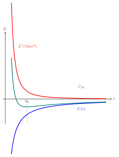
\[\boxed{U_{\rm eff}(r)=U(r)+\frac{L^2}{2mr^2}.}\]
第二项称为角动量势垒或离心势项;它来自角向动能在固定 \(L\) 下的重写,不是一个新的基本相互作用势。
4.2 Circular orbit and radial stability
径向方程为
\[m\ddot r=-\frac{dU_{\rm eff}}{dr}.\]
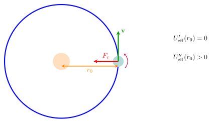
固定 \(L\) 的圆轨道要求
\[\dot r=0, \qquad \frac{dU_{\rm eff}}{dr}\bigg|_{r_0}=0.\]
对径向小扰动:
\[U_{\rm eff}''(r_0)>0\]
表示该圆轨道在固定角动量约束下径向稳定;小径向振动频率为
\[\omega_r=\sqrt{\frac{U_{\rm eff}''(r_0)}{m}}.\]
4.3 Worked Example 4 — harmonic central potential with angular momentum
取中心势
\[U(r)=\frac12kr^2,\]
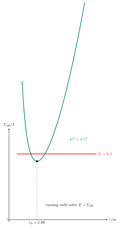
其中 \(m=2.00\ \mathrm{kg}\)、\(k=8.00\ \mathrm{N/m}\)、\(L=4.00\ \mathrm{kg\,m^2/s}\)。有效势为
\[U_{\rm eff}(r)=\frac12kr^2+\frac{L^2}{2mr^2}.\]
圆轨道条件:
\[\frac{dU_{\rm eff}}{dr}=kr-\frac{L^2}{mr^3}=0,\]
\[r_0=\left(\frac{L^2}{mk}\right)^{1/4} =1.00\ \mathrm m.\]
在此处
\[U_{\rm eff}(r_0) =\frac12(8.00)(1.00)^2 +\frac{4.00^2}{2(2.00)(1.00)^2} =8.00\ \mathrm J.\]
曲率为
\[U_{\rm eff}''(r) =k+\frac{3L^2}{mr^4},\]
\[U_{\rm eff}''(r_0)=8.00+24.0=32.0\ \mathrm{N/m}>0.\]
所以圆轨道径向稳定,且
\[\omega_r=\sqrt{\frac{32.0}{2.00}} =4.00\ \mathrm{rad/s}.\]
4.4 Applicability boundaries
有效势法在以下条件下成立:中心力、角动量守恒、用固定 \(L\) 比较径向运动。若存在非中心力、外力矩、阻力或显含时间的驱动,则 \(L\) 或 \(E\) 可变,单一静态 \(U_{\rm eff}(r)\) 不能完整描述过程。即使有效势给出 \(r(t)\) 的可达范围,仍要由
\[\dot\phi=\frac{L}{mr^2}\]
恢复角向演化,才能得到真实轨道。
5. Lesson synthesis / 全课整合
5.1 Landscape-reading algorithm
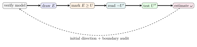
- 核实是一维保守运动,或已正确约化成单自由度。
- 统一能量零点,画 \(U(q)\) 和总能量 \(E\)。
- 用 \(E\ge U\) 标可达域,以 \(E=U\) 找候选转折点。
- 用 \(\dot q=\pm\sqrt{2(E-U)/m}\) 求速率,并由初值选方向。
- 用 \(F=-U'\) 判断加速度方向;检查 \(E=U\) 处是否同时 \(U'=0\)。
- 在 \(U'=0\) 处分类稳定性;若 \(U''=0\),检查更高阶项。
- 对非退化极小值,利用局部曲率估算小振动频率。
- 有效势问题还需写出守恒量来源并恢复被约化的角向运动。
5.2 What a landscape can and cannot tell
| Can infer directly | Cannot infer without more work |
|---|---|
| allowed regions, turning candidates, speed magnitude | direction branch without initial condition |
| equilibrium locations and local stability class | full time history \(q(t)\) |
| bound versus escape possibilities at fixed energy | behavior when energy changes through drive or dissipation |
| small-oscillation frequency near a nondegenerate minimum | large-amplitude period without nonlinear integration |
| radial behavior from \(U_{\rm eff}\) at fixed \(L\) | complete orbit without integrating \(\phi(t)\) |
6. Misconception clinic / 易错概念诊所
| Misconception / 错误观念 | Correction / 修正 |
|---|---|
| “势能图的纵轴是实际高度。” | 纵轴是能量;只有特定重力问题才与几何高度成正比。 |
| “\(U>E\) 区域只是速度为负。” | 它要求负动能,经典上不可达。 |
| “所有 \(E=U\) 点都会反弹。” | 若同时 \(U'=0\),可能是平衡点或渐近分离轨道。 |
| “极小值处动能一定为零。” | 只有静止在平衡时如此;穿过势阱底部的粒子动能常最大。 |
| “\(U''=0\) 表示中性平衡。” | 二阶判据无结论;\(x^4\)、\(-x^4\) 与常数势给出不同结果。 |
| “稳定平衡永远不会逃离。” | 局部稳定只针对足够小扰动;越过势垒需要足够能量。 |
| “任何势阱都严格简谐。” | 只有小振幅、非退化极小值附近的二次近似近似简谐。 |
| “二次项前的系数就是 \(U''\)。” | Taylor 项是 \(\tfrac12U''\xi^2\),要注意因子 \(1/2\)。 |
| “有效势中的离心项是新的基本力。” | 它是固定角动量下角向动能的径向重写。 |
| “得到 \(r(t)\) 就得到完整轨道。” | 还需积分 \(\dot\phi=L/(mr^2)\)。 |
7. Formula sheet / 公式表
| Concept | Equation | Conditions |
|---|---|---|
| Energy equation | \(E=\tfrac12m\dot x^2+U(x)\) | one-dimensional conservative motion |
| Accessible region | \(E\ge U(x)\) | classical \(K\ge0\) |
| Speed | \(\lvert\dot x\rvert=\sqrt{2[E-U(x)]/m}\) | choose direction separately |
| Equilibrium | \(U'(x_0)=0\) | \(F(x_0)=0\) |
| Nondegenerate stable point | \(U''(x_0)>0\) | local minimum |
| Small-oscillation frequency | \(\omega=\sqrt{U''(x_0)/m}\) | small amplitude, single mode |
| Effective potential | \(U_{\rm eff}=U(r)+L^2/(2mr^2)\) | central force, fixed \(L\) |
| Circular orbit | \(U_{\rm eff}'(r_0)=0\) | \(\dot r=0\) |
| Radial stability | \(U_{\rm eff}''(r_0)>0\) | fixed-\(L\) radial perturbation |
8. Practice and retrieval / 练习与检索
A. Conceptual questions
- 为什么 \(E-U\) 的竖直间隔代表动能而不是速度?
- 一个候选转折点同时满足 \(U'=0\) 时,为什么需要额外分析?
- 给出一个 \(U''(0)=0\) 但稳定的势,以及一个同样二阶导为零但不稳定的势。
- 小振动频率为什么由势阱曲率而不是势能绝对值决定?
- 有效势法为什么必须注明固定角动量?
B. Quantitative and derivation questions
- \(U(x)=\tfrac12(20.0\ \mathrm{N/m})x^2\),\(m=0.500\ \mathrm{kg}\),\(E=0.900\ \mathrm J\)。求转折点和 \(x=0\) 处速率。
- \(U(x)=ax^4-bx^2\),\(a,b>0\)。求所有平衡点并分类。
- 某势阱在 \(x_0\) 附近为 \(U=U_0+(18.0\ \mathrm{J/m^2})(x-x_0)^2\),质量 \(m=4.00\ \mathrm{kg}\)。求 \(\omega\) 与 \(T\)。
- 说明 \(U(x)=U_0+cx^4\)(\(c>0\))为何稳定,却不能用 \(\sqrt{U''(0)/m}\) 得到非零小振动频率。
- 对引力势 \(U=-GMm/r\),写出 \(U_{\rm eff}\) 并由极值条件求圆轨道半径与 \(L\) 的关系。
- 对本课 harmonic central potential 例题,若 \(E=9.00\ \mathrm J\),写出求径向转折点的方程。
Answers / 参考答案
1. \(E-U=K=\tfrac12mv^2\);速度还需平方根和方向分支。
2. 此处力也为零,可能是平衡或分离轨道端点,不一定有限时间反弹。
3. \(+ax^4\) 稳定,\(-ax^4\) 不稳定,二者在原点二阶导均为零。
4. 常数势能不产生力;恢复力线性系数是 \(U''(x_0)\)。
5. 角动量项来自用守恒 \(L\) 消去 \(\dot\phi\);若 \(L\) 改变,同一 \(U_{\rm eff}\) 不再适用。
6.
\[x_t=\pm\sqrt{\frac{2E}{k}}=\pm0.300\ \mathrm m,
\qquad
v(0)=\sqrt{\frac{2E}{m}}=1.90\ \mathrm{m/s}.\]
7. \(x=0\) 为极大值、不稳定;\(x=\pm\sqrt{b/(2a)}\) 为极小值、稳定。
8. \(U''=36.0\ \mathrm{N/m}\),\(\omega=3.00\ \mathrm{rad/s}\),\(T=2.09\ \mathrm s\)。
9. \(x=0\) 是严格极小值,但曲率为零,主导恢复力为 \(-4cx^3\),周期依振幅且不满足线性简谐公式。
10.
\[U_{\rm eff}=-\frac{GMm}{r}+\frac{L^2}{2mr^2},
\qquad
r_0=\frac{L^2}{GMm^2}.\]
11. 以 \(r\) 用米计,\(U_{\rm eff}=4r^2+4/r^2\) 焦耳,所以 \(4r^2+4/r^2=9\);令 \(z=r^2\) 得 \(4z^2-9z+4=0\)。
Exit ticket
画一个含局部极小、局部极大和逃逸方向的 \(U(x)\),放置三条不同总能量线;逐条标出可达域、普通转折点、可能的分离能量以及对应稳定性。
9. References and source notes / 参考资料与使用说明
9.1 Source-to-content map
| Source | Used for |
|---|---|
| OpenStax, University Physics Volume 1, §8.4 Potential Energy Diagrams and Stability | accessible regions, turning points, equilibrium classification and double-well reading |
| OpenStax, Chapter 8 Key Equations | energy and force-potential notation cross-check |
| MIT OpenCourseWare 8.03SC, Textbook Chapter 1: Harmonic Oscillation | Taylor expansion about equilibrium, linearity and small-oscillation frequency |
| MIT OCW 8.01SC, Chapter 25: Celestial Mechanics | angular-momentum barrier, effective potential, circular orbit and radial stability |
| MIT OpenCourseWare 8.09, Classical Mechanics III — Lecture Notes | advanced cross-check for small oscillations and central-force reduction boundaries |
9.2 Bibliographic notes
OpenStax §8.4 provides the potential-diagram spine. MIT 8.03SC supplies the local Taylor argument for harmonic behavior; MIT 8.01SC and 8.09 cross-check the effective-potential construction and its fixed-angular-momentum scope.