
Learning objectives / 学习目标
完成本课后,你应当能够:
- 用约束 Jacobian 的秩计算自由度,并区分完整、非完整、定常与随时间变化的约束。
- 从嵌入映射 \(\mathbf r_a(\mathbf q,t)\) 写出实际速度和固定时刻的虚位移。
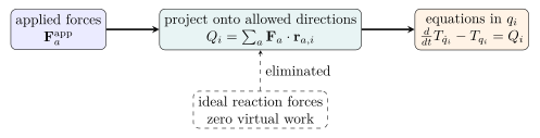
- 在“理想约束”前提下由达朗贝尔原理消去约束反力,并构造广义力。
- 精确表述 Hamilton's principle:真实轨迹使作用量 stationary / 驻定,不保证取得最小值。
- 在固定端点与适当正则性条件下,由一阶变分推导 Euler–Lagrange 方程。
- 对摆、Atwood machine 与旋转圆环等系统选择坐标、写出 \(L\) 并检查 SI 量纲。
0. Notation, dimensions, and logical route / 记号、量纲与逻辑路线
对 \(N\) 个质点,用 \(a=1,\ldots,N\) 标记粒子;每个 \(\mathbf r_a\in\mathbb R^3\)。用 \(i,j=1,\ldots,n\) 标记独立广义坐标。
| Symbol | Meaning | SI dimension |
|---|---|---|
| \(\mathbf r_a\) | particle position / 粒子位置 | m |
| \(q_i\) | generalized coordinate / 广义坐标 | depends on choice |
| \(\delta q_i\) | virtual change at fixed time / 固定时刻虚变分 | same as \(q_i\) |
| \(Q_i\) | generalized force conjugate to \(q_i\) | \(\mathrm J/[q_i]\) |
| \(L\) | Lagrangian / 拉格朗日量 | J |
| \(S=\int L\,dt\) | action / 作用量 | \(\mathrm{J\,s}\) |
| \(p_i=\partial L/\partial\dot q_i\) | generalized momentum / 广义动量 | \(\mathrm{J\,s}/[q_i]\) |
Knowledge 1 — Degrees of freedom and holonomic constraints / 自由度与完整约束
Knowledge ID: P01-U09-L01-K01
1.1 Degrees of freedom are local independent directions
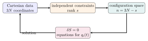
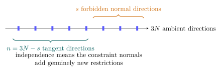
在无约束三维空间中,\(N\) 个质点有 \(3N\) 个位置坐标。若有 \(s\) 个彼此独立的完整约束
\[f_\alpha(\mathbf r_1,\ldots,\mathbf r_N,t)=0, \qquad \alpha=1,\ldots,s,\]
并且约束 Jacobian 对位置变量的秩为 \(s\),则在正则点附近12
\[\boxed{n=3N-s}\]
个独立参数足以标记所有允许构型。这个结论是局部的:若 Jacobian 降秩、坐标图出现极点或约束面自交,就必须换坐标图或重新分析。
1.2 Holonomic, scleronomous, rheonomous, and nonholonomic
- Holonomic / 完整约束: 可写成有限个 \(f_\alpha(\mathbf r,t)=0\),因此允许构型形成配置空间中的子流形。
- Scleronomous / 定常约束: \(f_\alpha\) 不显含 \(t\)。
- Rheonomous / 随动约束: \(f_\alpha\) 显含 \(t\),配置空间本身随时间移动。
- Nonholonomic / 非完整约束: 速度关系不能积分为只含坐标和时间的约束;平面上方向可变的圆盘或球的无滑动滚动通常是标准例子。特殊的一维纯滚动关系则可以积分,不能笼统地把所有“无滑动”都判作非完整。
速度形式
\[\sum_i a_{\alpha i}(\mathbf q,t)\dot q_i+a_{\alpha t}(\mathbf q,t)=0\]
只有在相应微分形式可积时才等价于完整约束。不能因为它“看起来是一阶线性的”就自动称为 holonomic。
Worked Example 1 — A bead constrained to a circular wire
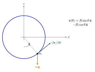
一颗珠子在竖直平面内沿半径 \(R\) 的固定圆环运动。用平面直角坐标 \((x,z)\) 描述时,有
\[f(x,z)=x^2+z^2-R^2=0.\]
环境维数为 2,独立约束数为 1,因此 \(n=1\)。可取
\[x=R\sin\theta,\qquad z=-R\cos\theta.\]
在 \(R=0.400\ \mathrm m\)、\(\theta=30.0^\circ\) 时,
\[(x,z)=(0.200,-0.346)\ \mathrm m.\]
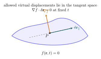
约束梯度 \((2x,2z)\) 与切向量
\[\frac{\partial\mathbf r}{\partial\theta} =(R\cos\theta,R\sin\theta)\]
点积为零,直接验证了允许方向与约束法向正交。
Knowledge 2 — Generalized coordinates and virtual displacement / 广义坐标与虚位移
Knowledge ID: P01-U09-L01-K02
2.1 The embedding map
解开完整约束后,把粒子位置写成
\[\boxed{\mathbf r_a=\mathbf r_a(q_1,\ldots,q_n,t)}.\]
对真实运动取全导数:
\[\boxed{ \dot{\mathbf r}_a =\sum_{i=1}^{n}\frac{\partial\mathbf r_a}{\partial q_i}\dot q_i +\frac{\partial\mathbf r_a}{\partial t} }.\]
最后一项只在嵌入显含时间时出现,例如被外部电机匀速转动的轨道。
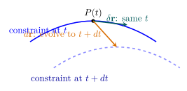
2.2 Virtual displacement is not an infinitesimal time step
在同一时刻 \(t\) 比较两个相邻允许构型:
\[\boxed{ \delta\mathbf r_a =\sum_i\frac{\partial\mathbf r_a}{\partial q_i}\delta q_i }, \qquad \delta t=0.\]
而真实的微分位移是
\[d\mathbf r_a =\sum_i\frac{\partial\mathbf r_a}{\partial q_i}dq_i +\frac{\partial\mathbf r_a}{\partial t}dt.\]
因此对 rheonomous constraint,\(\delta\mathbf r_a\) 与 \(d\mathbf r_a\) 一般不同。虚位移是“允许方向的比较”,不是粒子在 \(dt\) 内真的走过的路。
2.3 Configuration space
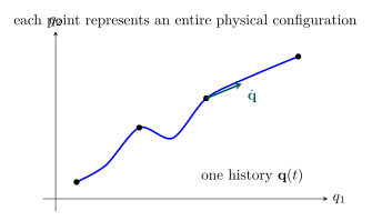
一个瞬时构型对应 \(\mathbf q=(q_1,\ldots,q_n)\) 的一个点;整个运动对应配置空间 \(\mathcal Q\) 中的一条曲线。注意:
- configuration space 不是普通三维空间;
- 两个质点在三维空间通常给出六维配置空间;
- 坐标图可能有奇点,但物理构型本身不一定奇异。
2.4 Virtual work and generalized force
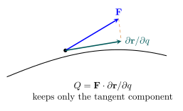
外力虚功可写成
\[\delta W =\sum_a\mathbf F_a\cdot\delta\mathbf r_a =\sum_i Q_i\,\delta q_i,\]
其中
\[\boxed{ Q_i=\sum_a\mathbf F_a\cdot \frac{\partial\mathbf r_a}{\partial q_i} }.\]
这一定义自动完成“把真实力投影到允许方向”。若 \(q_i\) 是角度,\(Q_i\) 就是相应轴的广义力矩。
Knowledge 3 — D'Alembert's principle / 达朗贝尔原理
Knowledge ID: P01-U09-L01-K03
3.1 Newton's law recast as virtual work
把 Newton 方程写成
\[\mathbf F_a^{\rm app}+\mathbf R_a-m_a\ddot{\mathbf r}_a=0,\]
其中 \(\mathbf R_a\) 是约束反力。与任意允许虚位移点乘并求和:
\[\sum_a \left( \mathbf F_a^{\rm app}+\mathbf R_a-m_a\ddot{\mathbf r}_a \right)\cdot\delta\mathbf r_a=0.\]
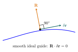
若约束是理想约束,
\[\sum_a\mathbf R_a\cdot\delta\mathbf r_a=0,\]
于是得到达朗贝尔原理:
\[\boxed{ \sum_a \left( \mathbf F_a^{\rm app}-m_a\ddot{\mathbf r}_a \right)\cdot\delta\mathbf r_a=0 }.\]
3.2 Kinetic-energy identity
对 \(\mathbf r_a(\mathbf q,t)\) 与
\[T=\frac12\sum_a m_a\dot{\mathbf r}_a^2,\]
可由链式法则证明
\[\sum_a m_a\ddot{\mathbf r}_a\cdot \frac{\partial\mathbf r_a}{\partial q_i} = \frac{d}{dt}\left(\frac{\partial T}{\partial\dot q_i}\right) -\frac{\partial T}{\partial q_i}.\]
代入达朗贝尔原理:
\[\sum_i \left[ Q_i-\frac{d}{dt}\left(\frac{\partial T}{\partial\dot q_i}\right) +\frac{\partial T}{\partial q_i} \right]\delta q_i=0.\]
对已经解开完整约束的独立 \(q_i\),各 \(\delta q_i\) 可独立选择,故
\[\boxed{ \frac{d}{dt}\left(\frac{\partial T}{\partial\dot q_i}\right) -\frac{\partial T}{\partial q_i}=Q_i }.\]
3.3 Conservative and nonconservative forces
若施加力来自势能 \(V(\mathbf q,t)\),
\[Q_i^{\rm cons}=-\frac{\partial V}{\partial q_i}.\]
令 \(L=T-V\),得到
\[\frac{d}{dt}\left(\frac{\partial L}{\partial\dot q_i}\right) -\frac{\partial L}{\partial q_i}=Q_i^{\rm nc}.\]
右端只保留不能纳入 \(L\) 的非保守广义力。粘滞力也可在某些线性模型中用 Rayleigh dissipation function 处理,但那不是 Hamilton principle 本身的一部分。
Worked Example 2 — The nonlinear pendulum
取摆角 \(\theta\) 自最低点量起:
\[T=\frac12m\ell^2\dot\theta^2, \qquad V=mg\ell(1-\cos\theta),\]
所以
\[L=\frac12m\ell^2\dot\theta^2-mg\ell(1-\cos\theta).\]
Euler–Lagrange 方程给出
\[m\ell^2\ddot\theta+mg\ell\sin\theta=0, \qquad \boxed{\ddot\theta=-\frac{g}{\ell}\sin\theta}.\]
若 \(\ell=0.800\ \mathrm m\)、\(\theta=30.0^\circ\),
\[\ddot\theta =-\frac{9.81}{0.800}\sin30.0^\circ =-6.13\ \mathrm{rad\,s^{-2}}.\]
质量消去不是遗漏;重力矩与转动惯量都正比于 \(m\)。
Knowledge 4 — Action and Hamilton's principle / 作用量与哈密顿原理
Knowledge ID: P01-U09-L01-K04
4.1 Action is a functional of an entire path
固定 \(t_1,t_2\),作用量定义为
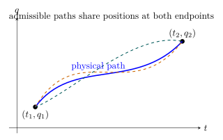
\[\boxed{ S[\mathbf q]=\int_{t_1}^{t_2} L(\mathbf q,\dot{\mathbf q},t)\,dt }.\]
\(S\) 的输入不是某一时刻的数,而是一整条路径 \(\mathbf q(t)\)。它的 SI 单位是 \(\mathrm{J\,s}\)。
构造相邻可容许路径
\[q_i^{(\varepsilon)}(t) =q_i(t)+\varepsilon\eta_i(t), \qquad \eta_i(t_1)=\eta_i(t_2)=0.\]
固定端点意味着所有比较路径在两个端时刻具有相同坐标;并不要求它们的端点速度相同。
4.2 Hamilton's principle means stationary action
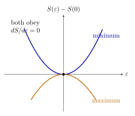
Hamilton's principle states
\[\boxed{ \delta S \equiv \left.\frac{d}{d\varepsilon} S[\mathbf q+\varepsilon\boldsymbol\eta] \right|_{\varepsilon=0} =0 }\]
for every admissible \(\boldsymbol\eta(t)\).
4.3 Scope and regularity
本课的标准推导假定:
- \(L(q,\dot q,t)\) 对其变量至少有足够连续的偏导,通常取 \(C^2\);
- 候选轨迹分段 \(C^2\),变分函数分段 \(C^1\);
- 两端时刻和两端位置固定;
- 所有完整约束已由独立坐标解开,或以一致的 Lagrange multiplier 方法加入;
- 运动没有冲击造成的速度跃变。
若端点可移动,会出现 natural boundary conditions;若轨迹分段光滑,角点还必须满足 Weierstrass–Erdmann matching conditions。这些不是标准固定端点式可以自动忽略的细节。
Knowledge 5 — Euler–Lagrange equations / 欧拉—拉格朗日方程
Knowledge ID: P01-U09-L01-K05
5.1 First variation and integration by parts
由
\[\delta\dot q_i=\frac{d}{dt}\delta q_i\]
得到
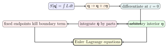
\[\delta S =\int_{t_1}^{t_2} \sum_i \left( \frac{\partial L}{\partial q_i}\delta q_i +\frac{\partial L}{\partial\dot q_i}\delta\dot q_i \right)dt.\]
对第二项分部积分:
\[\delta S = \left[ \sum_i\frac{\partial L}{\partial\dot q_i}\delta q_i \right]_{t_1}^{t_2} + \int_{t_1}^{t_2} \sum_i \left[ \frac{\partial L}{\partial q_i} -\frac{d}{dt} \left( \frac{\partial L}{\partial\dot q_i} \right) \right]\delta q_i\,dt.\]
固定端点使边界项为零。由变分法基本引理,若积分对所有内部任意的 \(\delta q_i\) 都为零,则
\[\boxed{ \frac{d}{dt} \left( \frac{\partial L}{\partial\dot q_i} \right) -\frac{\partial L}{\partial q_i}=0, \qquad i=1,\ldots,n }.\]
5.2 Equivalent Lagrangians
若
\[L'(\mathbf q,\dot{\mathbf q},t) =L(\mathbf q,\dot{\mathbf q},t) +\frac{dF(\mathbf q,t)}{dt},\]
则
\[S'=S+F(\mathbf q_2,t_2)-F(\mathbf q_1,t_1).\]
固定端点下附加项不变,因此 \(L\) 与 \(L'\) 给出同一 Euler–Lagrange 方程。Lagrangian 不是唯一的;物理内容在运动方程,而不在某个孤立的 \(L\) 表达式。
Worked Example 3 — Atwood machine without solving the tension
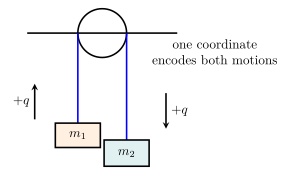
令 \(m_2>m_1\),取 \(q\) 为 \(m_2\) 向下的位移。绳不可伸长使另一块质量同时向上移动 \(q\);系统只有一个自由度。
\[T=\frac12(m_1+m_2)\dot q^2, \qquad V=(m_1-m_2)gq.\]
所以
\[L=\frac12(m_1+m_2)\dot q^2+(m_2-m_1)gq.\]
Euler–Lagrange 方程直接给出
\[\boxed{ \ddot q=\frac{m_2-m_1}{m_1+m_2}g }.\]
对 \(m_1=2.00\ \mathrm{kg}\)、\(m_2=3.00\ \mathrm{kg}\),
\[\ddot q=\frac{1.00}{5.00}(9.81) =1.962\ \mathrm{m\,s^{-2}}.\]
绳张力并未“消失”;它是理想约束的内部反力,对允许的成对位移总虚功为零。
Worked Example 4 — Bead on a uniformly rotating vertical hoop
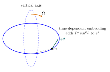
半径 \(R\) 的竖直圆环绕竖直直径以恒定角速度 \(\Omega\) 转动。以最低点为 \(\theta=0\):
\[\mathbf r= \left( R\sin\theta\cos\Omega t,\, R\sin\theta\sin\Omega t,\, -R\cos\theta \right).\]
由显含时间的嵌入求速度:
\[v^2=R^2\dot\theta^2+R^2\Omega^2\sin^2\theta.\]
于是
\[L= \frac12mR^2 \left( \dot\theta^2+\Omega^2\sin^2\theta \right) +mgR\cos\theta.\]
Euler–Lagrange 方程为
\[\boxed{ \ddot\theta =\sin\theta \left( \Omega^2\cos\theta-\frac{g}{R} \right) }.\]
取 \(R=0.500\ \mathrm m\)、\(\Omega=6.00\ \mathrm{rad\,s^{-1}}\)、\(\theta=10.0^\circ\):
\[\ddot\theta =\sin10.0^\circ \left[ (6.00)^2\cos10.0^\circ-\frac{9.81}{0.500} \right] =2.75\ \mathrm{rad\,s^{-2}}.\]
正号说明在该位置小珠被驱离最低点;最低点的线性稳定性阈值为 \(\Omega^2=g/R\)。
6. Lesson synthesis / 全课整合
6.1 The complete derivation chain
\[\boxed{ \begin{aligned} &f_\alpha(\mathbf r,t)=0 \quad\Longrightarrow\quad \mathbf r_a=\mathbf r_a(\mathbf q,t),\\ &\delta\mathbf r_a =\sum_i\frac{\partial\mathbf r_a}{\partial q_i}\delta q_i,\\ &\sum_a \left( \mathbf F_a^{\rm app}-m_a\ddot{\mathbf r}_a \right)\cdot\delta\mathbf r_a=0,\\ &Q_i= \frac{d}{dt} \left( \frac{\partial T}{\partial\dot q_i} \right) -\frac{\partial T}{\partial q_i},\\ &Q_i=-\frac{\partial V}{\partial q_i} \quad\Longrightarrow\quad \frac{d}{dt} \left( \frac{\partial L}{\partial\dot q_i} \right) -\frac{\partial L}{\partial q_i}=0. \end{aligned} }\]
Hamilton's principle reaches the same last line from a global path statement; D'Alembert reaches it from instantaneous virtual work. Their assumptions overlap strongly but their logical starting points are different.
6.2 Model-boundary checklist
| Question | If yes | If no |
|---|---|---|
| Can constraints be written as independent \(f_\alpha(\mathbf r,t)=0\)? | use \(n=3N-s\) locally | analyze nonholonomic or switching constraints |
| Do reaction forces do zero virtual work? | eliminate them by D'Alembert | retain their virtual work or use another contact model |
| Is the trajectory smooth and endpoints fixed? | standard variation applies | add corner or boundary conditions |
| Can applied forces be represented in \(L\)? | homogeneous Euler–Lagrange form | put \(Q_i^{\rm nc}\) on the right |
| Is the coordinate chart regular? | solve in that chart | change chart near singular points |
7. Misconception clinic / 易错概念诊所
| Misconception | Correction |
|---|---|
| “自由度等于写下的坐标数。” | 自由度是独立允许方向数;冗余坐标还要减去独立约束。 |
| “任何速度约束都能积分成坐标约束。” | 只有满足可积条件的速度关系才是 holonomic。 |
| “虚位移就是 \(d\mathbf r\)。” | 虚位移固定时间;rheonomous constraint 下二者不同。 |
| “达朗贝尔原理说约束力为零。” | 它要求理想约束力对允许虚位移总虚功为零。 |
| “作用量一定最小。” | 正确词是 stationary;\(\delta S=0\) 不决定二阶性质。 |
| “端点固定也固定端点速度。” | 标准变分只固定端点位置与时刻。 |
| “\(L\) 是唯一的物理能量。” | \(L\) 一般不是能量,且加全时间导数不改变运动方程。 |
8. Practice and retrieval / 练习与检索
A. Conceptual questions
- 两个质点在三维空间由一根不可伸长的轻杆连接,若没有其他约束,配置空间局部维数是多少?
- 为什么 \(\partial\mathbf r/\partial t\) 出现在真实速度中,却不出现在固定时刻的虚位移中?
- 一个粗糙固定曲面对滑块施加动摩擦,能否直接把接触力整体从达朗贝尔方程中消去?
- Hamilton's principle 为什么不能笼统翻译为“作用量最小”?
- 若 \(q=\theta\),为什么 \(Q_\theta\) 的 SI 单位不是 N?
- \(L\) 加上 \(dF/dt\) 后为何固定端点的运动方程不变?
B. Derivation and quantitative questions
- 从 \(\mathbf r=R(\cos\theta,\sin\theta)\) 证明圆环约束的虚位移与法向力正交。
- 对质量 \(m\) 的粒子在平面极坐标中运动,\(L=\frac12m(\dot r^2+r^2\dot\phi^2)-V(r,\phi)\)。推导两条 Euler–Lagrange 方程。
- Atwood machine 中 \(m_1=1.50\ \mathrm{kg}\)、\(m_2=2.50\ \mathrm{kg}\)。求加速度。
- 长度 \(\ell=1.20\ \mathrm m\) 的单摆在 \(\theta=20.0^\circ\) 处瞬时静止。求该瞬间角加速度与切向加速度。
- 证明若 \(L'=L+dF(q,t)/dt\),则两者的 Euler–Lagrange 表达式完全相同。
- 对旋转圆环,在 \(\theta\ll1\) 下线性化并判定 \(\Omega^2<g/R\) 与 \(\Omega^2>g/R\) 时最低点的稳定性。
Answers / 参考答案
1. 原有 6 个位置坐标,杆长给一个独立完整约束,所以局部自由度为 \(6-1=5\)。
2. 真实运动同时改变时间与坐标;虚位移比较同一时刻的相邻允许构型,定义上 \(\delta t=0\)。
3. 不能。法向部分对切向虚位移不做功,但动摩擦沿切向,虚功一般非零,必须作为施加广义力保留。
4. \(\delta S=0\) 只使一阶变化为零,可能是最小、最大或鞍型;要判断需看二阶变分。
5. \(Q_\theta\,d\theta\) 必须是功;弧度无量纲,所以 \(Q_\theta\) 的单位是 J,也就是 \(\mathrm{N\,m}\)。
6. 作用量只增加固定端点值 \(F(q_2,t_2)-F(q_1,t_1)\),其变分为零。
7.
\[\delta\mathbf r
=R(-\sin\theta,\cos\theta)\delta\theta,
\qquad
\mathbf R=R_n(\cos\theta,\sin\theta),\]
因而 \(\mathbf R\cdot\delta\mathbf r=0\)。
8.
\[m\ddot r-mr\dot\phi^2+\frac{\partial V}{\partial r}=0,\]
\[\frac{d}{dt}(mr^2\dot\phi)+\frac{\partial V}{\partial\phi}=0.\]
9.
\[a=\frac{2.50-1.50}{2.50+1.50}(9.81)
=2.45\ \mathrm{m\,s^{-2}}.\]
10.
\[\ddot\theta=-\frac{9.81}{1.20}\sin20.0^\circ
=-2.80\ \mathrm{rad\,s^{-2}},\]
\[a_t=\ell\ddot\theta=-3.36\ \mathrm{m\,s^{-2}}.\]
11. 展开 \(dF/dt=F_q\dot q+F_t\);代入 \(d(L'_{\dot q})/dt-L'_q\) 后,\(dF_q/dt-F_{qq}\dot q-F_{qt}=0\),附加项逐项抵消。多坐标情形相同。
12.
\[\ddot\theta
\simeq
\left(
\Omega^2-\frac{g}{R}
\right)\theta.\]
系数为负时是小振动、最低点线性稳定;系数为正时扰动指数增长、最低点不稳定;等号处线性项消失,线性化本身不能定论。
Exit ticket
不查公式,用五句话回答:
- 完整约束怎样减少自由度?
- 实际位移与虚位移有何不同?
- 达朗贝尔原理消去约束力的必要条件是什么?
- Hamilton's principle 的端点和“驻定”各指什么?
- Euler–Lagrange 方程中的边界项为何消失?
9. References and source notes / 参考资料与使用说明
9.1 Source-to-content map
| Source | Used for |
|---|---|
| MIT OCW 8.09 — Chapter 1: A Review of Analytical Mechanics | generalized coordinates, stationary action, constraints, D'Alembert principle, generalized force, Euler–Lagrange derivation |
| MIT OCW 8.09 — course readings | official scope for holonomic/nonholonomic constraints and D'Alembert treatment |
| David Tong, University of Cambridge — The Lagrangian Formulation | holonomic constraints, Lagrange multipliers, generalized coordinates, action and applications |
| David Tong, University of Cambridge — Classical Dynamics HTML, Section 2 | accessible cross-check of the same Cambridge derivations and small-oscillation bridge |
| MIT OCW 8.09 — syllabus | undergraduate level, analytical-mechanics coverage and prerequisite context |
9.2 Bibliographic notes
- Stewart, I. and MIT 8.09 course staff. A Review of Analytical Mechanics. 作为本课公式与符号的主要公开核对源。
- Tong, D. Lectures on Classical Dynamics, Chapter 2: The Lagrangian Formulation. University of Cambridge DAMTP;用于对约束、作用量和 Lagrange multiplier 处理作独立核对。
- 本文没有复制来源图形;所有 TikZ 图均由正文方程原创重绘。
注释与参考文献
MIT OpenCourseWare 8.09, Chapter 1: A Review of Analytical Mechanics.
↩David Tong, University of Cambridge DAMTP, The Lagrangian Formulation.
↩