
Learning objectives / 学习目标
完成本课后,你应当能够:
- 求 autonomous flow 的 fixed points,并用 Jacobian eigenvalues 作线性稳定性分类。
- 说明线性化对 nonhyperbolic fixed point 为什么可能失效,并区分 Lyapunov stable 与 asymptotically stable。
- 绘制 pendulum phase portrait,识别 center、saddle、libration、rotation 与 separatrix。
- 识别 saddle-node、transcritical、pitchfork 与 Hopf bifurcation 的基本特征。
- 从 harmonic balance 得到 Duffing response 的首阶振幅方程并解释弯曲与跳跃。
- 定义 finite-time 与 asymptotic Lyapunov exponent,避免把 deterministic chaos 等同于随机噪声。
- 构造 Poincaré section 和 return map,区分 periodic、quasiperiodic 与 chaotic signatures。
0. Dynamical-systems language / 动力系统语言
连续 autonomous system 写成
\[\boxed{ \dot{\mathbf x}=\mathbf F(\mathbf x;\mu) },\]
离散 map 写成
\[\boxed{ \mathbf x_{n+1}=\mathbf f(\mathbf x_n;\mu) }.\]
\(\mu\) 是 control parameter。时间连续流的 Jacobian eigenvalues 记为 \(\lambda_j\);离散 map 的线性乘子记为 \(\Lambda_j\),以免混淆稳定条件。
| Object | Continuous flow | Discrete map |
|---|---|---|
| fixed point | \(\mathbf F(\mathbf x_*)=0\) | \(\mathbf f(\mathbf x_*)=\mathbf x_*\) |
| linearization | \(\dot{\boldsymbol\xi}=\mathbf A\boldsymbol\xi\) | \(\boldsymbol\xi_{n+1}=\mathbf M\boldsymbol\xi_n\) |
| local stability | \(\operatorname{Re}\lambda_j<0\) | \(\lvert\Lambda_j\rvert<1\) |
| evolution | continuous trajectory | iterated sequence |
Knowledge 1 — Fixed points and stability / 不动点与稳定性
Knowledge ID: P01-U09-L04-K01
1.1 One-dimensional flows
对
\[\dot x=f(x),\]
不动点满足 \(f(x_*)=0\)。令 \(x=x_*+\xi\):
\[\dot\xi=f'(x_*)\xi+O(\xi^2).\]
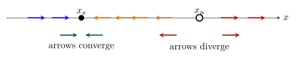
若 \(f'(x_*)\ne0\),
\[\xi(t)\simeq\xi(0)e^{f'(x_*)t}.\]
因此
\[\boxed{ f'(x_*)<0\Rightarrow\text{asymptotically stable}, \qquad f'(x_*)>0\Rightarrow\text{unstable} }.\]
若 \(f'(x_*)=0\),线性项不给答案,必须看更高阶项或构造 Lyapunov function。
1.2 Higher-dimensional Jacobian
在 \(\mathbf x_*\) 附近,
\[\dot{\boldsymbol\xi} =\mathbf A\boldsymbol\xi+O(\lVert\boldsymbol\xi\rVert^2), \qquad A_{ij} =\left. \frac{\partial F_i}{\partial x_j} \right|_{\mathbf x_*}.\]
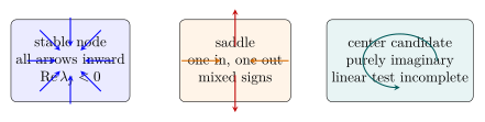
若 fixed point 是 hyperbolic,即所有 eigenvalues 都满足 \(\operatorname{Re}\lambda_j\ne0\):
- 全部 \(\operatorname{Re}\lambda_j<0\):sink / asymptotically stable;
- 全部 \(\operatorname{Re}\lambda_j>0\):source / unstable;
- 有正有负:saddle / unstable;
- 复共轭对的实部决定 spiral inward 或 outward。
纯虚 eigenvalues、零 eigenvalue 或 map multiplier 位于单位圆上时是 nonhyperbolic;非线性项可改变结论。
1.3 Lyapunov stability is not attraction
- Lyapunov stable: 对任意允许误差范围,都能选足够小的初始扰动,使轨迹永远留在该范围内。
- Asymptotically stable: Lyapunov stable,且邻近轨迹还满足 \(\mathbf x(t)\to\mathbf x_*\)。
- Hamiltonian oscillator 的 center 可 Lyapunov stable,却不会吸引邻近相轨线;Liouville theorem 禁止有限体积收缩成点。
Worked Example 1 — Supercritical pitchfork stability
考虑有量纲模型
\[\dot x=\mu x-\beta x^3, \qquad \beta>0.\]
fixed points:
\[x_0=0, \qquad x_\pm=\pm\sqrt{\frac{\mu}{\beta}} \quad(\mu>0).\]
因为
\[f'(x)=\mu-3\beta x^2,\]
所以 \(x_0\) 在 \(\mu<0\) 稳定、\(\mu>0\) 不稳定;\(x_\pm\) 在出现后满足 \(f'(x_\pm)=-2\mu<0\),稳定。
若 \(\mu=4.00\ \mathrm{s^{-1}}\)、\(\beta=1.00\ \mathrm{m^{-2}\,s^{-1}}\):
\[x_\pm=\pm2.00\ \mathrm m, \qquad f'(x_\pm)=-8.00\ \mathrm{s^{-1}}.\]
局部扰动按 \(e^{-8.00t}\) 衰减,e-folding time 为 \(0.125\ \mathrm s\)。
Knowledge 2 — Phase portraits and separatrices / 相图与分界轨道
Knowledge ID: P01-U09-L04-K02
2.1 Phase portrait
phase portrait 是状态空间中许多初值的轨线集合。对光滑 autonomous ODE,若解唯一,两条轨线不能在同一状态点相交;否则同一个初值会有两个未来。
2.2 Nonlinear pendulum
无阻尼摆:
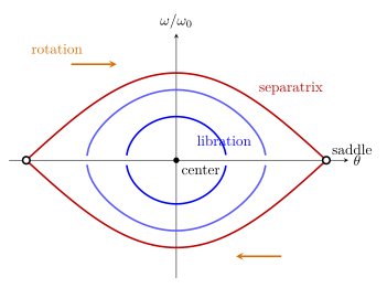
\[\dot\theta=\omega, \qquad \dot\omega=-\omega_0^2\sin\theta, \qquad \omega_0=\sqrt{\frac{g}{\ell}}.\]
每单位 \(m\ell^2\) 的守恒能量为
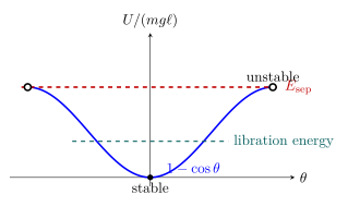
\[\boxed{ \mathcal H =\frac12\omega^2+\omega_0^2(1-\cos\theta) }.\]
fixed points:
\[(\theta,\omega)=(2k\pi,0) \quad\text{centers},\]
\[(\theta,\omega)=((2k+1)\pi,0) \quad\text{saddles}.\]
2.3 Separatrix
通过 saddle 的 stable/unstable manifolds 形成 separatrix。对摆,
\[\boxed{ \mathcal H_{\rm sep}=2\omega_0^2 }.\]
- \(\mathcal H<\mathcal H_{\rm sep}\):libration,轨线围绕 center 闭合;
- \(\mathcal H>\mathcal H_{\rm sep}\):rotation,\(\theta\) 连续增加或减少;
- \(\mathcal H=\mathcal H_{\rm sep}\):渐近接近倒立位置,理想模型中到达 saddle 需无限时间。
Worked Example 2 — Minimum bottom speed on the separatrix
在最低点 \(\theta=0\),separatrix condition 给
\[\frac12\omega^2=2\omega_0^2.\]
因此
\[\boxed{ \lvert\omega_{\rm bottom}\rvert=2\sqrt{\frac{g}{\ell}}, \qquad v_{\rm bottom}=2\sqrt{g\ell} }.\]
对 \(\ell=0.500\ \mathrm m\):
\[\lvert\omega_{\rm bottom}\rvert =8.86\ \mathrm{rad\,s^{-1}}, \qquad v_{\rm bottom}=4.43\ \mathrm{m\,s^{-1}}.\]
这是假设质点由刚性轻杆连接;若是只能拉不能推的细绳,还要检查绳张力非负,模型边界不同。
Knowledge 3 — Bifurcations and nonlinear resonance / 分岔与非线性共振
Knowledge ID: P01-U09-L04-K03
3.1 Bifurcation as a qualitative change
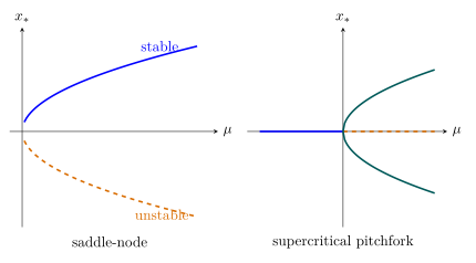
当 \(\mu\) 穿过临界值,fixed points、limit cycles 或其稳定性发生定性改变,称为 bifurcation。常见 normal forms:12
| Type | Normal form | Signature |
|---|---|---|
| saddle-node | \(\dot x=\mu-x^2\) | stable/unstable pair created or destroyed |
| transcritical | \(\dot x=\mu x-x^2\) | two branches exchange stability |
| supercritical pitchfork | \(\dot x=\mu x-x^3\) | one symmetric branch becomes two stable branches |
| Hopf | radial form \(\dot r=\mu r-r^3\) | fixed point exchanges stability with a limit cycle |
这些 normal forms 是局部模型;真实系统需满足相应非退化条件与对称性。pitchfork 在破坏反演对称性的微扰下通常会 unfold。
3.2 Duffing oscillator and harmonic balance
考虑受迫 Duffing equation:
\[\boxed{ \ddot x+2\gamma\dot x+\omega_0^2x+\alpha_Dx^3 =f\cos\omega t },\]
其中 \(f=F_0/m\)。设稳态主谐波
\[x(t)\simeq A\cos(\omega t-\delta),\]
并用
\[\cos^3u=\frac34\cos u+\frac14\cos3u\]
舍去三次谐波。比较同相与正交分量:
\[\boxed{ f^2 =A^2 \left[ \left( \omega_0^2-\omega^2+\frac34\alpha_DA^2 \right)^2 +(2\gamma\omega)^2 \right] },\]
为避免普通 \(\arctan\) 丢失象限信息,应把相位支固定为 \(0\le\delta\le\pi\),并写成
\[\boxed{ \delta=operatorname{atan2} \left( 2\gamma\omega, \omega_0^2-\omega^2+\frac34\alpha_DA^2 \right) }.\]
只有在另行判断分母符号与象限后,才可把它缩写成相应的 \(\tan\delta\) 关系。
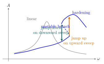
- \(\alpha_D>0\):hardening,resonance 向高频弯;
- \(\alpha_D<0\):softening,向低频弯;
- 足够强驱动时振幅方程可有多个解,出现 hysteresis 与 jump;不是每条代数支路都稳定。
Worked Example 3 — Amplitude-dependent frequency shift
对无阻尼、弱非线性、自由 Duffing oscillator,
\[\omega(A) \simeq \omega_0+\frac{3\alpha_DA^2}{8\omega_0}.\]
取
\[\omega_0=10.0\ \mathrm{rad\,s^{-1}}, \quad \alpha_D=200\ \mathrm{m^{-2}\,s^{-2}}, \quad A=0.0500\ \mathrm m.\]
则
\[\Delta\omega =\frac{3(200)(0.0500)^2}{8(10.0)} =1.875\times10^{-2}\ \mathrm{rad\,s^{-1}}.\]
所以 \(\omega\simeq10.019\ \mathrm{rad\,s^{-1}}\)。小参数
\[\frac{\alpha_DA^2}{\omega_0^2}=5.00\times10^{-3}\]
确实很小,与弱非线性展开一致。
Knowledge 4 — Deterministic chaos and Lyapunov exponents / 确定性混沌与李雅普诺夫指数
Knowledge ID: P01-U09-L04-K04
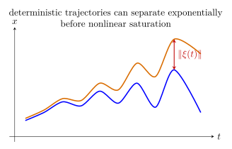
4.1 Sensitive dependence from the tangent dynamics
对参考轨迹 \(\mathbf x(t)\),邻近扰动满足一阶 variational equation:
\[\boxed{ \dot{\boldsymbol\xi} =\mathbf D\mathbf F[\mathbf x(t)] \boldsymbol\xi }.\]
令 \(\boldsymbol\Phi^t\) 为流映射,\(\mathbf D\boldsymbol\Phi^t(\mathbf x_0)\) 为其切向映射。最大渐近 Lyapunov exponent 可用最大奇异值写成3
\[\boxed{ \lambda_{\max}(\mathbf x_0) =\limsup_{t\to\infty} \frac1t \ln \sigma_{\max} \!\left[ \mathbf D\boldsymbol\Phi^t(\mathbf x_0) \right] }.\]
给定某个非零初始扰动方向 \(\boldsymbol\xi_0\),相应方向指数则是
\[\lambda(\mathbf x_0,\boldsymbol\xi_0) =\limsup_{t\to\infty} \frac1t \ln \frac{\lVert\mathbf D\boldsymbol\Phi^t(\mathbf x_0)\boldsymbol\xi_0\rVert} {\lVert\boldsymbol\xi_0\rVert} \le\lambda_{\max}.\]
在通常的正则性条件下,generic direction 配合周期性归一化会选出最大指数;但若 \(\boldsymbol\xi_0\) 恰落在较小指数的不变子空间中,上式不能冒充 \(\lambda_{\max}\)。
有限观测时间 \(T\) 给出
\[\boxed{ \lambda_T =\frac1T \ln \frac{\lVert\boldsymbol\xi(T)\rVert} {\lVert\boldsymbol\xi(0)\rVert} }.\]
\(\lambda_T\) 会随初值、方向和时间窗波动;只有适当极限及数值收敛分析后,才能把它解释为 asymptotic exponent。
4.2 Operational meaning and limits
对 bounded invariant set,最大渐近 exponent 为正是 deterministic chaos 的核心操作判据之一。常见对比:
| Long-time behavior | Typical largest exponent |
|---|---|
| stable fixed point | negative |
| autonomous stable limit cycle | zero; all transverse exponents are negative |
| quasiperiodic motion | zero exponents along neutral phase directions |
| chaotic trajectory | positive |
若初始不确定度为 \(\delta_0\)、容许误差为 \(\Delta\),粗略 predictability horizon 为
\[t_{\rm pred} \simeq \frac1{\lambda_{\max}} \ln\frac{\Delta}{\delta_0}.\]
4.3 Logistic map
采用 conventional logistic map
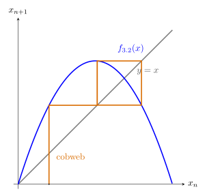
\[\boxed{ x_{n+1}=f_r(x_n)=rx_n(1-x_n), \qquad 0\le r\le4, \qquad x_0\in[0,1]\Longrightarrow x_n\in[0,1] }.\]
一维 map 的 finite-time exponent 是
\[\boxed{ \lambda_N =\frac1N \sum_{n=0}^{N-1} \ln\lvert f_r'(x_n)\rvert =\frac1N \sum_{n=0}^{N-1} \ln\lvert r(1-2x_n)\rvert }.\]
Worked Example 4 — Fixed-point stability and a chaotic exponent
nonzero fixed point 是
\[x_*=1-\frac1r,\]
其 multiplier
\[\Lambda=f_r'(x_*)=2-r.\]
- \(r=2.80\):\(\Lambda=-0.80\),fixed point stable;
- \(r=3.20\):\(\Lambda=-1.20\),fixed point unstable,系统进入 stable period-2 regime。
对 \(r=4\),几乎所有非特殊初值的理论 exponent 是
\[\lambda=\ln2=0.693147\ldots \quad\text{per iteration}.\]
从 \(x_0=0.123456789\) 出发,丢弃 1000 次 transient 后对 10000 次迭代求和,独立复算得
\[\lambda_{10000}=0.69320 \quad\text{per iteration},\]
与 \(\ln2\) 的差约 \(5.4\times10^{-5}\)。有限精度 logistic iteration 最终可能落入计算机的周期轨道,因此这只是有限窗数值核对,不是严格极限证明。
Knowledge 5 — Poincaré sections and routes to chaos / 庞加莱截面与通往混沌的道路
Knowledge ID: P01-U09-L04-K05
5.1 Reducing a flow to a return map
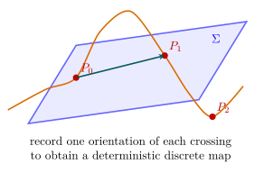
在 \(d\) 维 flow 中选一个 transversal surface
\[\Sigma:\ h(\mathbf x)=0,\]
并只记录同一穿越方向,例如
\[\dot h=\nabla h\cdot\mathbf F>0.\]
连续轨迹与 \(\Sigma\) 的交点形成序列4
\[\boxed{ \mathbf X_{n+1}=\mathcal P(\mathbf X_n) },\]
\(\mathcal P\) 称 Poincaré return map。截面通常把维数降低 1;若还固定 autonomous Hamiltonian 的能量,两个自由度系统的三维能量壳可得到二维截面。
对周期受迫系统,也常每隔 drive period \(T_d\) 取样:
\[t_n=t_0+nT_d.\]
这叫 stroboscopic section;若取样周期与驱动周期不一致,图样会产生人为漂移。
5.2 Reading a section
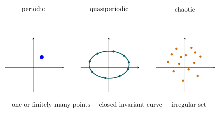
- periodic orbit:一个点或有限个点;
- quasiperiodic motion:通常落在闭合 invariant curve 上;
- chaotic motion:不规则点集。耗散系统可形成 fractal strange attractor;保守系统常出现 chaotic sea 与 regular islands 共存。
5.3 Routes to chaos
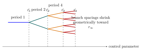
常见路线包括:5
- Period doubling: 周期 \(1\to2\to4\to8\to\cdots\);
- Intermittency: 长时间近规则段被不规则 burst 打断;
- Quasiperiodicity: 多个不可公度频率经 torus breakdown 进入混沌。
对 conventional logistic map,前两个倍周期阈值为
\[r_1=3, \qquad r_2=1+\sqrt6=3.449489\ldots,\]
并在
\[r_\infty\simeq3.569946\]
附近积聚。若 \(r_n\) 是 successive thresholds,
\[\boxed{ \delta =\lim_{n\to\infty} \frac{r_n-r_{n-1}}{r_{n+1}-r_n} =4.669201\ldots }.\]
Feigenbaum universality 需要 map 峰值附近具有合适的 quadratic maximum 等条件;它不是所有通往 chaos 的普适常数。
Worked Example 5 — Interpreting a driven-pendulum section
对
\[\ddot\theta+2\gamma\dot\theta+\omega_0^2\sin\theta =f\cos\Omega t,\]
每隔
\[T_d=\frac{2\pi}{\Omega}\]
记录 \((\theta\bmod2\pi,\dot\theta)\):
- 一个点表示与 drive 同周期的稳定响应;
- 两个交替点表示 period-2 response;
- 闭曲线表示 quasiperiodic response;
- 收敛后的不规则 fractal set 加上正的 converged \(\lambda_{\max}\) 支持 chaotic attractor 判断。
若 \(\Omega=3.00\ \mathrm{rad\,s^{-1}}\),则
\[T_d=\frac{2\pi}{3.00}\ \mathrm s \simeq2.094\ \mathrm s.\]
实际采样始终使用
\[t_n=t_0+n\left(\frac{2\pi}{3.00}\right)\mathrm s;\]
\(2.094\ \mathrm s\) 只作显示近似,不能在长序列中反复累加这个舍入值。还必须固定同一个 \(t_0\bmod T_d\),否则无法定义单一 return map。
6. Lesson synthesis / 全课整合
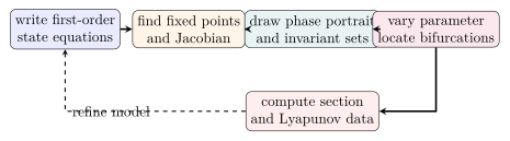
6.1 Analysis workflow
6.2 Model boundaries that must travel with the conclusion
| Conclusion | Required boundary |
|---|---|
| linear stability from eigenvalues | hyperbolic fixed point or separate nonlinear analysis |
| separatrix classification | autonomous conservative pendulum model |
| Duffing amplitude curve | weak harmonic-balance truncation and steady periodic response |
| positive Lyapunov exponent | converged long-time tangent dynamics on the relevant invariant set |
| Poincaré signature | fixed section, fixed crossing orientation, transients removed |
| Feigenbaum scaling | appropriate unimodal map universality class |
7. Misconception clinic / 易错概念诊所
| Misconception | Correction |
|---|---|
| “Jacobian 有纯虚 eigenvalues 就证明稳定。” | 这是 nonhyperbolic case,非线性项可能决定稳定或不稳定。 |
| “center 是 asymptotically stable。” | 保守 center 可 Lyapunov stable,但不吸引相邻轨线。 |
| “phase-portrait 轨线永远不能交叉。” | 完整 autonomous state space 中不交叉;丢掉 drive phase 的投影可交叉。 |
| “separatrix 是有限时间到达 saddle 的普通轨道。” | 理想 autonomous model 中通常渐近接近,所需时间发散。 |
| “nonlinear resonance 只有一个振幅。” | 强驱动 Duffing response 可多值,且只有部分支路稳定。 |
| “有限时间正 Lyapunov exponent 就证明 chaos。” | 必须检查时间窗、transient、bounded set 与渐近收敛。 |
| “chaos 就是随机。” | chaos 由确定方程生成;随机过程的不可预测性来源不同。 |
| “Poincaré 云越乱越 chaotic。” | 噪声、aliasing 和错误采样也会产生云,需独立诊断。 |
8. Practice and retrieval / 练习与检索
A. Conceptual questions
- 为什么 \(f'(x_*)=0\) 时不能用一维线性稳定性公式下结论?
- Hamiltonian center 为什么不能吸引一个有限面积的邻域?
- pendulum separatrix 在相图中分隔哪两类运动?
- pitchfork bifurcation 为什么通常需要对称性保护?
- \(\lambda_T>0\) 与 \(\lambda_{\max}>0\) 的逻辑差别是什么?
- 为什么 Poincaré section 只记录一个穿越方向?
- smooth autonomous two-dimensional flow 为什么不能拥有 strange attractor,而 two-dimensional map 可以表现 chaos?
B. Derivation and quantitative questions
- 对 \(\dot x=\mu-x^2\) 求 fixed points 与稳定性,并画 bifurcation branches。
- 对 pendulum separatrix 推导 \(\omega(\theta)=\pm2\omega_0\cos(\theta/2)\),取 \(-\pi\le\theta\le\pi\)。
- 对 logistic map 证明 nonzero fixed point 在 \(1<r<3\) 稳定。
- 初始误差 \(\delta_0=10^{-9}\)、容许误差 \(\Delta=10^{-2}\)、\(\lambda_{\max}=0.40\ \mathrm{s^{-1}}\)。估算 predictability horizon。
- Duffing oscillator 取 \(\alpha_D<0\),说明 resonance curve 弯向哪一侧。
- period-4 orbit 在 stroboscopic Poincaré section 中应出现几个点?
- 若 map 的一周期 multiplier 为 \(-1.2\),该 fixed point 是否稳定?最可能发生哪类局部分岔?
Answers / 参考答案
1. 线性项消失,高阶项与全局结构成为 leading order;不同非线性项可给相反结论。
2. Liouville theorem 保持 canonical phase area;吸引整个邻域到一点会把非零面积压成零。
3. 内部是绕稳定平衡的 libration,外部是持续 rotation;边界通过倒立 saddle。
4. 对称性保证中央支路与成对分支;小的不对称项一般把理想 pitchfork 展开成 saddle-node 类型结构。
5. \(\lambda_T\) 是特定有限窗平均,可能受 transient 与方向影响;\(\lambda_{\max}\) 是适当长时间极限。
6. 若正反穿越都混在一起,return map 不再对应单一的“下一次同向返回”,会人为叠加两张 map。
7. 在标准光滑性、boundedness 与有限 fixed-point 等假设下,Poincaré–Bendixson structure 限制二维连续 autonomous flow 的极限集;离散 map 不受该连续流拓扑限制。
8.
\[x_\pm=\pm\sqrt{\mu}
\quad(\mu>0),
\qquad
f'(x)=-2x.\]
因而 \(x_+\) 稳定、\(x_-\) 不稳定;\(\mu<0\) 无 fixed point,\(\mu=0\) 为 nonhyperbolic collision。
9.
\[\frac12\omega^2+\omega_0^2(1-\cos\theta)
=2\omega_0^2,\]
\[\omega^2
=2\omega_0^2(1+\cos\theta)
=4\omega_0^2\cos^2(\theta/2).\]
在指定区间 \(\cos(\theta/2)\ge0\),故得两支 \(\omega=\pm2\omega_0\cos(\theta/2)\)。
10.
\[x_*=1-\frac1r,
\qquad
\Lambda=f'(x_*)=2-r.\]
\(\lvert2-r\rvert<1\) 给 \(1<r<3\)。
11.
\[t_{\rm pred}
=\frac1{0.40}\ln\frac{10^{-2}}{10^{-9}}
=40.3\ \mathrm s.\]
12. \(\alpha_D<0\) 使振幅增大时有效频率降低,response curve 向低频侧弯。
13. 四个循环点;每次取样依次访问一个点。
14. 不稳定,因为 \(\lvert\Lambda\rvert>1\);若 multiplier 由单位圆内穿过 \(-1\),典型是 flip 或 period-doubling bifurcation。
Exit ticket
用一页草图完成:
- 一个 center 与一个 saddle 的相图;
- 一条 separatrix;
- 一个 pitchfork diagram;
- 两条初值接近而指数分离的轨迹;
- periodic、quasiperiodic、chaotic 三类 Poincaré signatures。
9. References and source notes / 参考资料与使用说明
9.1 Source-to-content map
| Source | Used for |
|---|---|
| MIT OCW 8.09 — Chapter 7: Chaos and Non-Linear Dynamics | fixed points, phase portraits, bifurcation normal forms, limit cycles, maps and chaos overview |
| MIT OCW 12.006J — Lectures 2–3: Flows and Bifurcations in One Dimension | one-dimensional flow stability, saddle-node and transcritical bifurcations |
| MIT OCW 12.006J — Lectures 4–5: Pendulum and Stability in Two-Dimensional Systems | pendulum phase portrait, fixed-point classification and two-dimensional stability |
| MIT OCW 12.006J — Lectures 15–16: Poincaré Sections | construction, crossing direction, return maps and periodic/quasiperiodic/aperiodic signatures |
| MIT OCW 12.006J — Lecture 24: Lyapunov Exponents | tangent dynamics, exponent definition, numerical renormalization and interpretation |
| MIT OCW 12.006J — Lectures 25–27: Period Doubling Route to Chaos | period-doubling cascade, logistic-map thresholds and Feigenbaum scaling |
| MIT OCW 12.006J — lecture-notes index | official course provenance and links to all topic-specific notes |
9.2 Bibliographic notes
- Stewart, I. and MIT 8.09 course staff. Chaos and Non-Linear Dynamics. 用作 advanced undergraduate analytical-mechanics 主干。
- Rothman, D. H. and MIT 12.006J course staff. Nonlinear Dynamics: Chaos lecture notes. 用于对 bifurcations、Poincaré sections、Lyapunov exponents 和 period doubling 作逐项独立核对。
- 所有相图、函数图与分岔图均依据正文方程原创绘制,没有复制来源图像。
注释与参考文献
MIT OpenCourseWare 8.09, Chapter 7: Chaos and Non-Linear Dynamics.
↩MIT OpenCourseWare 12.006J, Lectures 2–3: Flows and Bifurcations in One Dimension.
↩MIT OpenCourseWare 12.006J, Lecture 24: Lyapunov Exponents.
↩MIT OpenCourseWare 12.006J, Lectures 15–16: Poincaré Sections.
↩MIT OpenCourseWare 12.006J, Lectures 25–27: Period Doubling Route to Chaos.
↩