
Learning objectives / 学习目标
- 从独立对称随机步推导均方位移和 diffusion coefficient,并说明 diffusion limit 的尺度条件。
- 写出 underdamped 与 overdamped Langevin equation,识别 friction、deterministic force 与 noise。
- 从 stochastic differential equation 对应到 Fokker–Planck probability current,并检验归一化和 stationary distribution。
- 使用 Einstein 与 noise-friction 形式的 fluctuation–dissipation relation,解释其平衡前提。
- 建立有限状态 continuous-time Markov master equation,求 stationary distribution、relaxation time 并判断 detailed balance。
Prerequisites / 先修知识
- 概率分布、期望值与微观态。
- Fick diffusion、mobility 与 Einstein relation。
- Gaussian integral、Taylor expansion、first-order linear ODE 和 probability normalization。
- Canonical distribution \(P_{\mathrm{eq}}\propto e^{-U/(k_BT)}\)。
Scope and conventions / 范围与约定
- \(P\) 始终表示 probability density 或 discrete probability,并满足归一化;\(c\) 才表示物质浓度。
- Wiener increment 采用 \(\langle dW\rangle=0\)、\(\langle(dW)^2\rangle=dt\) 的 convention。
- Langevin white noise 是 coarse-grained idealization,不代表真实分子力在任意短时间都无相关。
- 除特别说明外,热浴静止、温度均匀;friction coefficient \(\gamma>0\),potential force 为 \(F=-dU/dx\)。
- 本课主要使用 additive noise,因此不进入 Itô–Stratonovich ambiguity;multiplicative noise 只列为模型边界。
Notation and modeling contract / 符号与建模契约
| Symbol | Meaning | SI unit |
|---|---|---|
| \(a\) | random-walk step length | m |
| \(\tau_s\) | time per discrete step | s |
| \(D\) | diffusion coefficient | \(\mathrm{m^2\,s^{-1}}\) |
| \(P(x,t)\) | probability density | \(\mathrm{m^{-1}}\) |
| \(\gamma\) | translational friction coefficient | \(\mathrm{kg\,s^{-1}}\) |
| \(\xi(t)\) | stochastic force | N |
| \(A(x,t)\) | drift coefficient in an SDE | \(\mathrm{m\,s^{-1}}\) |
| \(B(x,t)\) | infinitesimal variance coefficient | \(\mathrm{m^2\,s^{-1}}\) |
| \(W_{ij}\) | transition rate from \(j\) to \(i\) | \(\mathrm{s^{-1}}\) |
| \(\tau_r\) | relaxation/correlation time | s |
Knowledge 1 — Random walks and diffusion limit / 随机游走与扩散极限
Knowledge ID: P03-U08-L02-K01
1.1 平均位移可以为零,均方位移仍然增长
一维对称随机游走每步 \(\Delta x_n=\pm a\),两方向概率各 \(1/2\)。经过 \(N\) 个独立步,
\[x_N-x_0=\sum_{n=1}^{N}\Delta x_n, \qquad \langle x_N-x_0\rangle=0.\]
独立性使 cross terms 平均为零:
\[\langle(x_N-x_0)^2\rangle =\sum_{n=1}^{N}\langle(\Delta x_n)^2\rangle =Na^2.\]
令 \(t=N\tau_s\),并定义
\[\boxed{D=\frac{a^2}{2\tau_s}},\]
就得到一维 Einstein law
\[\boxed{\langle\Delta x^2\rangle=2Dt.}\]
\(d\) 维各向同性情形为 \(\langle\lvert\Delta\mathbf r\rvert^2\rangle=2dDt\)。
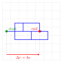
图 1:这条 20-step square-lattice realization 同时含前进与回退,每段长度为 \(a\),净位移 \(4a\) 与 rms scale \(\sqrt{20}a\) 同量级。二维图只展示几何;正文的一维模型把每一步严格限制为 \(\pm a\)。
1.2 Diffusion limit 是离散步长的 coarse-grained 极限
当观察尺度远大于 \(a\)、观察时间远大于 \(\tau_s\),并保持 \(a^2/(2\tau_s)=D\) 有限时,binomial distribution 趋向 Gaussian:
\[P(x,t)=\frac{1}{\sqrt{4\pi Dt}} \exp\left(-\frac{x^2}{4Dt}\right).\]
它满足 \(\partial_tP=D\partial_x^2P\)。这并不表示每个粒子沿 Gaussian 曲线运动;曲线描述 many-realization ensemble。
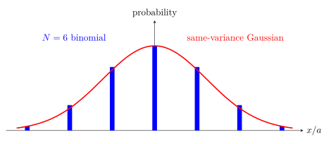
图 2:\(N=6\) 时柱高按 \(1:6:15:20:15:6:1\) 绘制并整体缩放;红线使用同一 variance \(Na^2\)。小 \(N\) 下近似仍粗糙,large-\(N\) coarse graining 才趋于 Gaussian。
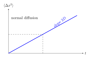
图 3:normal diffusion 的 MSD–time 图是过原点直线;ballistic 或 anomalous diffusion 会有不同幂律。
Worked Example 1 — 从步长得到 diffusion coefficient
已知: 一维粒子每 \(\tau_s=0.500\ \mathrm s\) 独立地向左或向右走 \(a=2.00\ \mathrm{\mu m}\)。求 \(N=100\) 步后的时间、rms displacement 和 continuum \(D\)。
研究对象与参考系: 实验室系中的单个 walker;统计量取大量同条件轨迹。
坐标: 右为 \(+x\)。
模型理由: 步长固定、方向等概率、步间无相关。
\[t=N\tau_s=50.0\ \mathrm s.\]
\[x_{\mathrm{rms}}=\sqrt{\langle\Delta x^2\rangle} =a\sqrt N=(2.00\ \mathrm{\mu m})(10.0) =20.0\ \mathrm{\mu m}.\]
\[D=\frac{a^2}{2\tau_s} =\frac{(2.00\times10^{-6})^2}{2(0.500)} =4.00\times10^{-12}\ \mathrm{m^2\,s^{-1}}.\]
检查 continuum relation:
\[\sqrt{2Dt}=20.0\ \mathrm{\mu m}.\]
检查: 平均位移为零不与非零 rms 冲突;\(a^2/\tau_s\) 单位为 \(\mathrm{m^2\,s^{-1}}\)。结果三位有效数字。
Knowledge 2 — Brownian motion and Langevin equation / 布朗运动与朗之万方程
Knowledge ID: P03-U08-L02-K02
2.1 一条随机动力学方程同时包含系统力、阻力和热浴噪声
一维 underdamped Langevin equation 为
\[\boxed{m\dot v=-\gamma v-U'(x)+\xi(t),\qquad \dot x=v.}\]
\(-\gamma v\) 是平均耗散力;\(\xi(t)\) 是热浴许多快速碰撞的 coarse-grained 随机合力。平衡 white-noise idealization 取
\[\langle\xi(t)\rangle=0, \qquad \langle\xi(t)\xi(t')\rangle =2\gamma k_BT\,\delta(t-t').\]
在 \(t\gg m/\gamma\) 的 overdamped limit,惯性项可消去:
\[\gamma\dot x=-U'(x)+\xi(t).\]
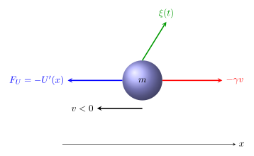
图 4:所选瞬间 \(v<0\),所以 drag \(-\gamma v\) 指向右;蓝箭头是 potential force \(-U'(x)\),绿色随机箭头只是一份瞬时样本。
自由粒子的 velocity autocorrelation 是
\[\langle v(t)v(0)\rangle =\frac{k_BT}{m}e^{-t/\tau_v}, \qquad \tau_v=\frac{m}{\gamma}.\]
短时 \(t\ll\tau_v\) 近似 ballistic,长时才进入 \(\langle\Delta x^2\rangle\approx2Dt\)。
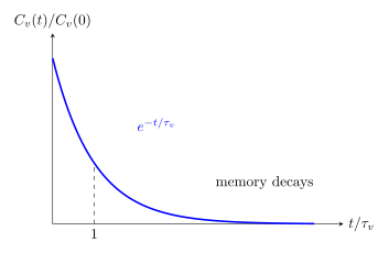
图 5:Markovian friction 下的 velocity correlation 以 \(\tau_v=m/\gamma\) 衰减。
Worked Example 2 — 水中微球的 Stokes–Einstein diffusion
已知: 半径 \(r=0.500\ \mathrm{\mu m}\) 的球形粒子在 \(T=298\ \mathrm K\)、黏度 \(\eta=1.00\times10^{-3}\ \mathrm{Pa\,s}\) 的无限液体中运动。求 \(\gamma=6\pi\eta r\)、\(D\),以及一维 rms displacement 达 \(10.0\ \mathrm{\mu m}\) 的时间。
系统与参考系: 稀释单球,远处流体静止。
坐标: 任取一维投影。
模型理由: low Reynolds number、no slip、远离边界,使用 Stokes drag 和 equilibrium Einstein relation。
\[\gamma=6\pi\eta r =6\pi(1.00\times10^{-3})(0.500\times10^{-6}) =9.42\times10^{-9}\ \mathrm{kg\,s^{-1}}.\]
\[D=\frac{k_BT}{\gamma} =\frac{(1.380649\times10^{-23})(298)} {9.42\times10^{-9}} =4.37\times10^{-13}\ \mathrm{m^2\,s^{-1}}.\]
由 \(\langle\Delta x^2\rangle=2Dt\),
\[t=\frac{(10.0\times10^{-6})^2}{2D} =1.14\times10^2\ \mathrm s.\]
检查: \(\gamma\) 单位满足 \(F=\gamma v\);更大 \(r\) 或 \(\eta\) 使 \(D\) 变小。时间是 ensemble rms 条件,不是每个粒子首次到达时间。结果三位有效数字。
Knowledge 3 — Fokker–Planck equation / 福克—普朗克方程
Knowledge ID: P03-U08-L02-K03
3.1 从随机轨迹转到 probability current
对 Itô SDE
\[dx=A(x,t)\,dt+\sqrt{B(x,t)}\,dW,\]
相应 Fokker–Planck equation 为
\[\boxed{ \frac{\partial P}{\partial t} =-\frac{\partial}{\partial x}(AP) +\frac12\frac{\partial^2}{\partial x^2}(BP). }\]
若 \(B=2D\) 为常数,可写成 probability conservation:
\[\frac{\partial P}{\partial t}+\frac{\partial J_P}{\partial x}=0, \qquad J_P=AP-D\frac{\partial P}{\partial x}.\]
适当的 zero-flux 或 decaying boundary condition 保证 \(\int P\,dx=1\)。
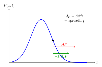
图 6:虚线所示点位于峰右侧,故 \(\partial_xP<0\),diffusive current \(-D\partial_xP\) 指向 \(+x\);红、绿箭头在同一局部位置分层画出。
3.2 Harmonic trap 给出 Ornstein–Uhlenbeck process
对 \(U(x)=\kappa x^2/2\) 的 overdamped Brownian particle,
\[A(x)=-\frac{\kappa}{\gamma}x, \qquad D=\frac{k_BT}{\gamma}.\]
零流 stationary solution 是
\[P_{\mathrm{eq}}(x) =\sqrt{\frac{\kappa}{2\pi k_BT}} \exp\left(-\frac{\kappa x^2}{2k_BT}\right),\]
所以 \(\langle x^2\rangle_{\mathrm{eq}}=k_BT/\kappa\)。Fokker–Planck 描述 ensemble density;Langevin 描述一条 realization,二者不是竞争模型。
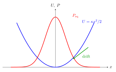
图 7:harmonic restoring drift 把 probability 拉回中心,而 diffusion 使分布展宽;平衡宽度由二者共同决定。
Worked Example 3 — Optical trap 中的 equilibrium variance
已知: 一维 harmonic trap stiffness \(\kappa=2.00\times10^{-6}\ \mathrm{N\,m^{-1}}\),\(T=300\ \mathrm K\),friction \(\gamma=1.00\times10^{-8}\ \mathrm{kg\,s^{-1}}\)。求平衡 rms displacement 和 overdamped relaxation time。
系统与参考系: 热浴中的 trapped particle,trap center 为 \(x=0\)。
模型理由: harmonic potential、constant \(\gamma\)、equilibrium additive white noise。
\[\langle x^2\rangle_{\mathrm{eq}} =\frac{k_BT}{\kappa} =\frac{(1.380649\times10^{-23})(300)} {2.00\times10^{-6}} =2.07\times10^{-15}\ \mathrm{m^2}.\]
\[\boxed{x_{\mathrm{rms}}=4.55\times10^{-8}\ \mathrm m =45.5\ \mathrm{nm}.}\]
Ornstein–Uhlenbeck mean relaxation time is
\[\boxed{\tau_r=\frac{\gamma}{\kappa} =5.00\times10^{-3}\ \mathrm s.}\]
检查: equipartition 给 \(\kappa\langle x^2\rangle/2=k_BT/2\),与 Fokker–Planck result 一致;更硬的 trap 使 variance 与 relaxation time 都减小。结果三位有效数字。
Knowledge 4 — Fluctuation–dissipation relation / 涨落—耗散关系
Knowledge ID: P03-U08-L02-K04
4.1 同一个热浴既产生阻力,也产生噪声
若保留 \(\gamma\) 却令 \(\xi=0\),粒子最终静止,不能维持温度 \(T\) 的 canonical equilibrium;若只加噪声而无阻力,能量无限增长。平衡要求二者配对:
\[\boxed{\langle\xi(t)\xi(t')\rangle =2\gamma k_BT\,\delta(t-t').}\]
长时间空间扩散则给
\[\boxed{D=\frac{k_BT}{\gamma}=bk_BT.}\]
这两式是 fluctuation–dissipation relation 的 Brownian forms:自发 equilibrium fluctuations 的强度决定线性耗散响应。
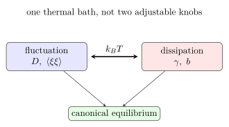
图 8:在 equilibrium Langevin model 中,noise amplitude 与 friction 不能独立选择。
4.2 适用边界
经典 form 要求 heat bath 处于平衡、response 足够弱、时间尺度分离允许 Markov/white-noise approximation。量子系统、colored noise、active matter 或 driven bath 需要 generalized relation;不能把 \(D=k_BT/\gamma\) 当作任何非平衡随机过程的定义。
Knowledge 5 — Markov processes and master equations / 马尔可夫过程与主方程
Knowledge ID: P03-U08-L02-K05
5.1 Markov property 与状态概率的守恒
Markov property 表示:给定现在状态后,未来条件概率不再依赖更早历史。对离散状态 continuous-time jump process,令 \(W_{ij}\) 是从 \(j\) 跳到 \(i\) 的 rate,则
\[\boxed{ \frac{dp_i}{dt} =\sum_{j\ne i}\left(W_{ij}p_j-W_{ji}p_i\right). }\]
第一项是 inflow,第二项是 outflow;求和可验证 \(\sum_i\dot p_i=0\)。Stationary distribution 满足 \(\dot p_i=0\)。Detailed balance 更强:
\[W_{ij}p_j^{\mathrm{eq}} =W_{ji}p_i^{\mathrm{eq}}\]
对每一对状态成立。Stationary 不必然 detailed balanced;非平衡稳态可有循环 probability current。
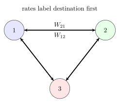
图 9:三态 Markov network;每条有向边是 probability flow channel,rate convention 必须先声明。
5.2 两态系统显示指数弛豫
两态 \(1\rightleftarrows2\),从 \(1\) 到 \(2\) 的 rate 为 \(k_{12}\)、反向为 \(k_{21}\):
\[\dot p_1=-k_{12}p_1+k_{21}p_2, \qquad p_2=1-p_1.\]
于是
\[p_1(t)=p_1^{\mathrm{ss}} +\left[p_1(0)-p_1^{\mathrm{ss}}\right] e^{-(k_{12}+k_{21})t},\]
\[p_1^{\mathrm{ss}}=\frac{k_{21}}{k_{12}+k_{21}}.\]
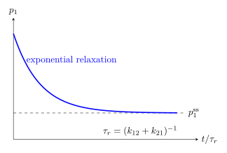
图 10:横轴是 dimensionless time \(t/\tau_r\),因此曲线含 \(e^{-t/\tau_r}\);两态 probability 从初值指数趋向 stationary value。
Worked Example 4 — 两态 master equation
已知: \(k_{12}=3.00\ \mathrm{s^{-1}}\)、\(k_{21}=1.00\ \mathrm{s^{-1}}\),初态 \(p_1(0)=1\)。求 stationary probabilities、relaxation time 和 \(t=0.500\ \mathrm s\) 时的 \(p_1\)。
系统边界: 封闭二态 probability ensemble,\(p_1+p_2=1\)。
时间参考: \(t=0\) 为制备在状态 1 的时刻。
模型理由: rates constant,过程 memoryless。
\[p_1^{\mathrm{ss}}=\frac{1}{3+1}=0.250, \qquad p_2^{\mathrm{ss}}=0.750.\]
\[\tau_r=\frac{1}{k_{12}+k_{21}} =0.250\ \mathrm s.\]
\[p_1(0.500) =0.250+0.750e^{-4(0.500)} =0.352.\]
Detailed-balance check:
\[p_1^{\mathrm{ss}}k_{12} =(0.250)(3.00) =(0.750)(1.00) =p_2^{\mathrm{ss}}k_{21}.\]
检查: 概率均在 \([0,1]\) 内且相加为 1;\(t\to\infty\) 回到 0.250。结果三位有效数字。
Lesson synthesis / 全课整合
随机过程有三个互补描述层次:
- trajectory level: random walk 或 Langevin equation 生成单条 realization;
- distribution level: Fokker–Planck 或 master equation 演化 ensemble probability;
- thermodynamic constraint: fluctuation–dissipation 与 detailed balance 决定哪些随机参数能代表温度为 \(T\) 的 equilibrium bath。
建模流程是:选状态变量与时间分辨率 → 判断 discrete/continuous、Markov/non-Markov → 写 drift、noise 或 transition rates → 推出 probability balance → 检查 normalization、stationary state、MSD/correlation 和 equilibrium constraint → 最后才把 ensemble prediction 与实验轨迹统计比较。
Formula-and-decision table / 公式—决策表
| Task | Relation | Use only when | Key caution |
|---|---|---|---|
| 1D walk MSD | \(\langle\Delta x^2\rangle=Na^2=2Dt\) | independent unbiased steps | mean displacement remains zero |
| \(d\)-D diffusion | \(\langle\lvert\Delta\mathbf r\rvert^2\rangle=2dDt\) | normal isotropic diffusion | not valid for anomalous exponent |
| underdamped Langevin | \(m\dot v=-\gamma v-U'+\xi\) | separated bath time scale | \(\xi\) is stochastic force |
| FDT noise | \(\langle\xi(t)\xi(t')\rangle=2\gamma k_BT\delta(t-t')\) | classical equilibrium white noise | bath and response assumptions required |
| Fokker–Planck | \(\partial_tP=-\partial_x(AP)+\frac12\partial_x^2(BP)\) | stated Itô SDE | multiplicative noise convention matters |
| probability current | \(J_P=AP-D\partial_xP\) | \(B=2D\) constant | boundary current controls normalization |
| Einstein relation | \(D=k_BT/\gamma\) | long-time equilibrium Brownian motion | walls and hydrodynamic memory modify drag |
| master equation | \(\dot p_i=\sum_{j\ne i}(W_{ij}p_j-W_{ji}p_i)\) | continuous-time Markov jumps | declare rate-index convention |
| detailed balance | \(W_{ij}p_j^{\mathrm{eq}}=W_{ji}p_i^{\mathrm{eq}}\) | equilibrium reversible network | stationarity alone is weaker |
Model boundaries / 模型边界
- Independence of steps fails with persistence, trapping, long-range correlations or Lévy flights; MSD may scale as \(t^\alpha\) with \(\alpha\ne1\).
- White noise requires bath correlation time much shorter than resolved system time; at shorter scales use colored noise or generalized Langevin memory kernels.
- Overdamped elimination requires \(t\gg m/\gamma\); it erases the ballistic short-time regime.
- Fokker–Planck with multiplicative noise requires an explicit stochastic-calculus convention.
- Markov coarse graining can fail if hidden slow variables retain memory.
- Detailed balance is an equilibrium property; driven chemical cycles and active matter can have stationary distributions with nonzero cycle currents.
- Classical FDT changes in quantum or strongly nonequilibrium baths.
Misconception clinic / 易错概念诊所
- “随机游走平均位移为零,所以粒子没有扩散。” 错;扩散由 variance 或 MSD 增长刻画。
- “Gaussian density 是一条典型粒子轨迹。” 错;它是 ensemble probability density。
- “Langevin equation 违反 Newton's law。” 错;它是未解析 bath degrees of freedom 后的 effective equation。
- “friction 越大,noise 应越小。” 错;固定 \(T\) 的 equilibrium FDT 要求 force-noise amplitude 随 \(\gamma\) 增大。
- “Fokker–Planck 和 Langevin 给出两个不同实验。” 错;在相同 convention 下,它们是 trajectory 与 distribution 的对应描述。
- “stationary 就等于 equilibrium。” 错;NESS 可 stationary 但有非零 probability currents 和 entropy production。
Practice and retrieval / 练习与检索
1. 随机游走 MSD(K01)
二维 square lattice 每步长 \(a\)、步间隔 \(\tau_s\),四方向等概率。写出 \(D\) 与 \(\langle r^2\rangle\)。
Answer
每步 \(\langle\Delta r^2\rangle=a^2\),而二维 normal diffusion 有 \(\langle r^2\rangle=4Dt\)。因此 \(D=a^2/(4\tau_s)\),\(N\) 步后 \(\langle r^2\rangle=Na^2\)。
2. Drifted walk(K01)
若一维每步向右概率 \(p\ne1/2\),求单步平均位移。
Answer
\(\langle\Delta x\rangle=pa+(1-p)(-a)=(2p-1)a\)。此时有 drift,不能只用零均值 diffusion kernel。
3. Ballistic 与 diffusive(K02)
自由 Langevin particle 在什么时间尺度下分别近似 \(\langle\Delta x^2\rangle\propto t^2\) 与 \(\propto t\)?
Answer
\(t\ll\tau_v=m/\gamma\) 时速度尚有记忆,近似 ballistic \(t^2\);\(t\gg\tau_v\) 时记忆消失,进入 \(2Dt\)。
4. Overdamped 条件(K02)
为什么不能在研究 \(t\sim m/\gamma\) 的实验时删去 \(m\dot v\)?
Answer
该时间正是惯性与摩擦竞争的 velocity-relaxation scale;删去惯性会错误消除 ballistic crossover 与 velocity correlation。
5. Fokker–Planck current(K03)
\(A=v_0\)、\(D\) 常数时写出 \(J_P\)。
Answer
\(J_P=v_0P-D\partial_xP\);第一项平移 distribution,第二项展宽 distribution。
6. Stationary harmonic density(K03)
为什么 equilibrium harmonic density 的 exponent 必须是 \(-\kappa x^2/(2k_BT)\)?
Answer
Canonical weight 为 \(e^{-U/(k_BT)}\),而 \(U=\kappa x^2/2\);也可令 Fokker–Planck current 为零并用 \(D=k_BT/\gamma\) 得到同式。
7. FDT 参数审计(K04)
模拟把 \(\gamma\) 加倍但保持 noise correlation amplitude 不变。长期 effective temperature 如何变化?
Answer
由 amplitude \(2\gamma k_BT\),若 amplitude 固定而 \(\gamma\) 加倍,则对应的 effective \(T\) 减半;模型不再代表原温度热浴。
8. Einstein relation(K04)
\(D=5.0\times10^{-13}\ \mathrm{m^2\,s^{-1}}\)、\(T=300\ \mathrm K\),求 \(\gamma\)。
Answer
\(\gamma=k_BT/D=(1.380649\times10^{-23})(300)/(5.0\times10^{-13})=8.3\times10^{-9}\ \mathrm{kg\,s^{-1}}\)。
9. Master-equation conservation(K05)
说明为什么每一条 \(j\to i\) 的 probability flow 不改变 \(\sum_i p_i\)。
Answer
它在 \(\dot p_i\) 中作为 \(+W_{ij}p_j\),同时在 \(\dot p_j\) 中作为等大的 outflow \(-W_{ij}p_j\);求和时逐边抵消。
10. Stationary vs detailed balance(K05)
三态环有稳定的顺时针 probability current。它能否满足 detailed balance?
Answer
不能。Stationarity 只要求每个节点总流入等于总流出;detailed balance 要求每一对边净流都为零。持续环流意味着非平衡稳态。
Exit ticket / 课末检验
- 给定一个 noisy trajectory,说明如何用 MSD、velocity correlation 与 stationary histogram 分别检验 \(D\)、\(\tau_v\) 和 potential model。
- 从 overdamped Langevin SDE 写出 Fokker–Planck current,并列出使 Boltzmann distribution 成为 zero-current equilibrium 所需的关系。
References and source notes / 参考资料与来源说明
- MIT OCW 5.72, Stochastic Processes and Brownian Motion — Markov process、master equation、Fokker–Planck、Langevin 与 Brownian applications。
- MIT OCW 8.334, Lecture 26 — Dissipative Dynamics — probability current、Fokker–Planck equation、Boltzmann stationary state 与 fluctuation–dissipation condition。
- MIT OCW 18.366, Lecture 14 — Random Walks and Diffusion — biased walk、Einstein relation、Smoluchowski equation 与 Ornstein–Uhlenbeck process。
- MIT OCW 2.57, Complete Lecture Notes — Nano-to-Macro Transport Processes — Langevin/Stokes–Einstein derivation and transport scale boundary。
- Jean Baptiste Perrin — Nobel Lecture, Discontinuous Structure of Matter — Brownian evidence、molecular interpretation 与历史实验边界。
- NIST CODATA Values of the Fundamental Physical Constants — exact \(k_B\) and SI numerical convention。
以上来源均于 2026-08-25 实际打开并核对到具体页面或 PDF。正文统一采用本文声明的 SDE、rate-index 和 SI conventions;图像均依据方程原创。
Source-to-content map
| Source | Used for | Knowledge ID / Section | Model boundary or convention |
|---|---|---|---|
| MIT 5.72 Chapter 1 | Markov, master, Fokker–Planck, Langevin | K02, K03, K05 | graduate notes adapted without importing advanced formalism |
| MIT 8.334 Lecture 26 | probability current and equilibrium stationary state | K03, K04 | additive diffusion and linear mobility |
| MIT 18.366 Lecture 14 | random-walk limit, Einstein and OU | K01–K04 | Itô SDE and Stokes low-Re condition made explicit |
| MIT 2.57 notes | Brownian transport scale and drag | K02, K04 | continuum hydrodynamic drag boundary retained |
| Perrin Nobel lecture | experimental meaning of Brownian statistics | K01, K02 | historical evidence, not used as sole derivation |
| NIST CODATA | numerical constants | Worked Examples 2–3, Practice 8 | exact SI \(k_B\) |
复习与拓展
- 下一课把 probability relaxation 与 macroscopic entropy production、Onsager symmetry 连接起来。
- Kinetic theory 会从 collision dynamics 求 effective friction、diffusion and transport coefficients。
- Quantum open systems 将把 classical white noise 换成 operator correlation 与 quantum FDT。
- Data analysis 可用 maximum likelihood、autocorrelation 和 hidden Markov models 从有限轨迹估计参数。