
Learning objectives / 学习目标
- 陈述 local-equilibrium hypothesis 的空间与时间尺度要求,并写出局域 entropy balance。
- 为 heat conduction、diffusion 与 chemical reaction 选择共轭 thermodynamic force/flux,使 entropy production 是 \(\sum_i\mathbf J_i\cdot\mathbf X_i\)。
- 使用线性 phenomenological matrix 判断 second-law positivity,并在满足 microscopic reversibility 时应用 Onsager 或 Onsager–Casimir relation。
- 区分 equilibrium、near-equilibrium transient 与 nonequilibrium steady state,正确核算 system、reservoirs 与 total entropy。
- 识别 far-from-equilibrium nonlinear response、instability 与 dissipative structure,并拒绝无条件套用极小或极大熵产生原理。
Prerequisites / 先修知识
- 熵平衡、Clausius inequality 与 entropy production。
- chemical potential 与 conjugate variables。
- Fick、Fourier、viscosity 与 mobility。
- detailed balance、fluctuation–dissipation 与 stationary probability current。
Scope and conventions / 范围与约定
- 先采用 local equilibrium:每个足够小但仍含大量粒子的 cell 具有 \(T(\mathbf r,t)\)、\(p(\mathbf r,t)\)、\(\mu_a(\mathbf r,t)\) 等局域强度量。
- Flux 均相对于声明的参考速度定义;多组分 diffusion 默认相对于 barycentric frame。
- Entropy-production density 记为 \(\sigma_s\),单位 \(\mathrm{W\,m^{-3}K^{-1}}\),并要求 \(\sigma_s\ge0\)。
- Linear irreversible thermodynamics 只用于接近平衡、局域力较小的范围。外磁场、旋转、奇偶 time-reversal parity 会修改简单的 \(L_{ij}=L_{ji}\)。
- “far from equilibrium”没有一个普适小参数;本课只建立边界意识和典型 bifurcation 图景,不声称存在通用封闭理论。
Notation and modeling contract / 符号与建模契约
| Symbol | Meaning | SI unit |
|---|---|---|
| \(s\) | entropy density | \(\mathrm{J\,m^{-3}K^{-1}}\) |
| \(\mathbf J_s\) | entropy-flux density | \(\mathrm{W\,m^{-2}K^{-1}}\) |
| \(\sigma_s\) | entropy-production rate density | \(\mathrm{W\,m^{-3}K^{-1}}\) |
| \(\mathbf q\) | heat-flux density | \(\mathrm{W\,m^{-2}}\) |
| \(\mathbf J_a\) | molar diffusion flux of species \(a\) | \(\mathrm{mol\,m^{-2}s^{-1}}\) |
| \(\mu_a\) | molar chemical potential | \(\mathrm{J\,mol^{-1}}\) |
| \(\mathbf X_i\) | thermodynamic force conjugate to \(\mathbf J_i\) | force-dependent |
| \(L_{ij}\) | phenomenological coefficient | pair-dependent |
| \(\mathcal A_r\) | molar affinity of reaction \(r\) | \(\mathrm{J\,mol^{-1}}\) |
| \(\mathcal R_r\) | volumetric reaction rate | \(\mathrm{mol\,m^{-3}s^{-1}}\) |
Knowledge 1 — Local equilibrium and entropy production / 局域平衡与熵产生
Knowledge ID: P03-U08-L03-K01
1.1 Local equilibrium 是尺度假设,不是“每处都已平衡”
设 microscopic correlation/mean-free-path scale 为 \(\ell_{\mathrm{micro}}\),macroscopic gradient scale 为 \(L_{\mathrm{grad}}\)。Local equilibrium 需要能选 cell size \(\ell_c\) 满足
\[\ell_{\mathrm{micro}}\ll\ell_c\ll L_{\mathrm{grad}},\]
并且 local relaxation time 远短于宏观演化时间。这样每个 cell 内可用 equilibrium equation of state,而 cell 之间仍有 \(T\)、\(\mu\) 等梯度,产生净 flux。
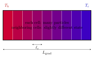
图 1:局域 cell 内可近似平衡,但跨越许多 cell 存在宏观温度梯度;颜色和 cell 数均为示意。
1.2 Entropy balance 区分输运与产生
局域 entropy balance 为
\[\boxed{ \frac{\partial s}{\partial t} +\nabla\cdot\mathbf J_s =\sigma_s,\qquad \sigma_s\ge0. }\]
\(-\nabla\cdot\mathbf J_s\) 描述 entropy 进出,不是局域产生;\(\sigma_s\) 才是 irreversible production。对控制体积 \(V\),
\[\frac{dS_V}{dt} =-\oint_{\partial V}\mathbf J_s\cdot d\mathbf A +\int_V\sigma_s\,dV.\]
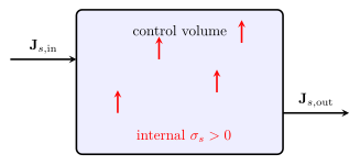
图 2:entropy 可随 flux 穿过边界,同时在内部产生;稳态只要求两者账本相抵。
对只导热的静止介质,\(\mathbf J_s=\mathbf q/T\),并可得
\[\boxed{ \sigma_s=\mathbf q\cdot\nabla\left(\frac1T\right) =\frac{k}{T^2}\lvert\nabla T\rvert^2\ge0. }\]
Worked Example 1 — 稳态导热的 entropy production
已知: 均匀平板 \(L=0.100\ \mathrm m\)、\(A=1.00\times10^{-2}\ \mathrm{m^2}\)、\(k=2.00\ \mathrm{W\,m^{-1}K^{-1}}\),热面 \(T_h=400\ \mathrm K\),冷面 \(T_c=300\ \mathrm K\)。求 steady heat rate 与 system+reservoirs 的 total entropy-production rate。
系统边界: 板加两个理想 reservoirs;板侧面绝热。
参考系与方向: 实验室系,热流从 hot 向 cold 为正。
模型理由: 一维、常 \(k\)、steady Fourier conduction。
\[\dot Q=\frac{kA(T_h-T_c)}{L} =\frac{(2.00)(1.00\times10^{-2})(100)}{0.100} =20.0\ \mathrm W.\]
板处于 steady state,\(dS_{\mathrm{plate}}/dt=0\)。两 reservoir 的 entropy rates 为 \(-\dot Q/T_h\) 与 \(+\dot Q/T_c\),所以
\[\dot S_{\mathrm{gen}} =\dot Q\left(\frac1{T_c}-\frac1{T_h}\right) =20.0\left(\frac1{300}-\frac1{400}\right) =1.67\times10^{-2}\ \mathrm{W\,K^{-1}}.\]
检查: 结果为正;若 \(T_h=T_c\),热流与 entropy production 同时归零。不能因板的 entropy 不变就声称过程可逆。三位有效数字。
Knowledge 2 — Thermodynamic forces and fluxes / 热力学力与流
Knowledge ID: P03-U08-L03-K02
2.1 共轭配对由 entropy production 决定
Irreversible thermodynamics 把 entropy production 写成 bilinear sum:
\[\boxed{ \sigma_s=\sum_i\mathbf J_i\cdot\mathbf X_i +\sum_r\mathcal R_r\frac{\mathcal A_r}{T}. }\]
典型配对是:
- heat flux \(\mathbf q\) 与 \(\nabla(1/T)\);
- diffusion flux \(\mathbf J_a\) 与 \(-\nabla(\mu_a/T)\);
- reaction rate \(\mathcal R_r\) 与 affinity \(\mathcal A_r/T\)。
Force 的定义不是任意“看起来像梯度”的量;必须让 product 具有 entropy-production density 的单位和正确 time-reversal structure。
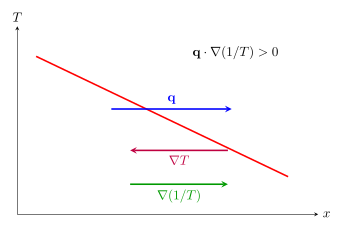
图 3:\(\mathbf q\) 与 \(\nabla T\) 反向,却与 \(\nabla(1/T)\) 同向,因此 entropy production 为正。
2.2 Linear phenomenological laws
Near equilibrium 时把 flux 对 forces 作一阶展开:
\[\boxed{\mathbf J_i=\sum_jL_{ij}\mathbf X_j.}\]
Diagonal coefficient 描述 direct effect;off-diagonal coefficient 描述 cross effect,如 temperature gradient 驱动 particle/electric current,或 chemical-potential gradient 伴随 heat flow。
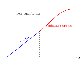
图 4:linear law 是 \(X=0\) 附近的一阶近似;驱动力大时曲线可饱和、弯曲或失稳。
Worked Example 2 — Isothermal ideal-solution diffusion 的 entropy production
已知: \(T=300\ \mathrm K\),一维薄层厚 \(L=1.00\ \mathrm{mm}\),两端 molar concentration \(c_L=2.00\ \mathrm{mol\,m^{-3}}\)、\(c_R=1.00\ \mathrm{mol\,m^{-3}}\),\(D=1.00\times10^{-9}\ \mathrm{m^2\,s^{-1}}\)。以 linear steady profile 求 flux,并用 ideal \(\mu=\mu^\circ+RT\ln(c/c^\circ)\) 估计平均 entropy-production density。
系统与参考系: 静止溶剂中的稀溶质,相对于 solvent frame;恒温、无反应。
坐标: \(+x\) 从左向右。
模型理由: 理想稀溶液、constant \(D\)、steady one-dimensional transport。
\[J_x=-D\frac{c_R-c_L}{L} =1.00\times10^{-6}\ \mathrm{mol\,m^{-2}s^{-1}}.\]
跨层的 molar \(\mu/T\) 变化为
\[\frac{\mu_R-\mu_L}{T} =R\ln\left(\frac{c_R}{c_L}\right) =-R\ln2.\]
故平均 thermodynamic force
\[X=-\frac{\Delta(\mu/T)}{L} =\frac{R\ln2}{L} =5.76\times10^3\ \mathrm{J\,mol^{-1}K^{-1}m^{-1}}.\]
\[\boxed{ \sigma_s=J_xX =5.76\times10^{-3}\ \mathrm{W\,m^{-3}K^{-1}}. }\]
检查: molar flux 乘 \(\mathrm{J\,mol^{-1}K^{-1}m^{-1}}\) 得 \(\mathrm{W\,m^{-3}K^{-1}}\);高浓度向低浓度扩散使 \(\sigma_s>0\)。强非理想溶液需 activity 与 thermodynamic factor。
Knowledge 3 — Onsager reciprocal relations / 昂萨格互易关系
Knowledge ID: P03-U08-L03-K03
3.1 Microscopic reversibility 约束 cross coefficients
在接近平衡、线性响应、正确选择 conjugate forces/fluxes 且无 time-reversal-breaking field 时,Onsager reciprocity 给
\[\boxed{L_{ij}=L_{ji}.}\]
它不是仅由第二律推出。第二律只要求 coefficient matrix 的对称部分 positive semidefinite,使
\[\sigma_s=\mathbf X^{\mathsf T}\mathbf L\mathbf X\ge0.\]
对 symmetric \(2\times2\) matrix,需
\[L_{11}\ge0,\qquad L_{22}\ge0,\qquad L_{11}L_{22}-L_{12}^2\ge0.\]
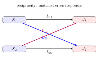
图 5:off-diagonal arrows 表示 coupled transport;互易性比较的是规范化后的共轭 pair。
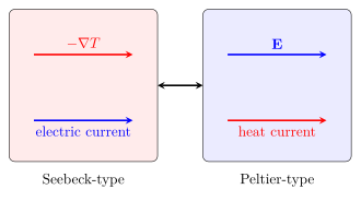
图 6:thermoelectric cross effects 是 reciprocal-coefficient 的典型应用;实际系数还受 convention 与 Kelvin relations 约束。
3.2 Onsager–Casimir correction
若存在 magnetic field \(\mathbf B\) 或 rotation,time reversal 同时反转这些量。更一般地,
\[\boxed{ L_{ij}(\mathbf B) =\epsilon_i\epsilon_jL_{ji}(-\mathbf B), }\]
其中 \(\epsilon_i=\pm1\) 是相应 variable 的 time-reversal parity。因而在固定非零 \(\mathbf B\) 下简单写 \(L_{ij}=L_{ji}\) 可能错误。
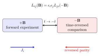
图 7:有磁场时互易比较必须同时反转 field,并跟踪变量的 time-reversal parity。
Worked Example 3 — 两组分 coupled diffusion matrix
已知: 两个 molar flux 的线性 law 为 \(\mathbf J=\mathbf L\mathbf X\),其中
\[\mathbf L=10^{-10} \begin{pmatrix} 4&1\\ 1&3 \end{pmatrix} \mathrm{mol^2\,K\,J^{-1}m^{-1}s^{-1}},\]
\[\mathbf X= \begin{pmatrix} 2.00\times10^3\\ -1.00\times10^3 \end{pmatrix} \mathrm{J\,mol^{-1}K^{-1}m^{-1}}.\]
求 fluxes 与 \(\sigma_s\),并检查 stability。
系统与参考系: 等温二组分介质,相对 barycentric frame。
模型理由: 近 equilibrium、同 time-reversal parity、constant symmetric \(\mathbf L\)。
\[J_1=10^{-10}\left[4(2000)+1(-1000)\right] =7.00\times10^{-7}\ \mathrm{mol\,m^{-2}s^{-1}},\]
\[J_2=10^{-10}\left[1(2000)+3(-1000)\right] =-1.00\times10^{-7}\ \mathrm{mol\,m^{-2}s^{-1}}.\]
\[\boxed{ \sigma_s=J_1X_1+J_2X_2 =1.50\times10^{-3}\ \mathrm{W\,m^{-3}K^{-1}}>0. }\]
Matrix minors 为 \(L_{11}>0\) 且
\[L_{11}L_{22}-L_{12}^2 =(12-1)\times10^{-20}>0,\]
故 positive definite。检查: \(J_2<0\) 并不违反第二律;只有总 bilinear entropy production 必须非负。单位逐项闭合。
Knowledge 4 — Steady states far from equilibrium / 远离平衡的稳态
Knowledge ID: P03-U08-L03-K04
4.1 Steady state 不等于 equilibrium
Nonequilibrium steady state, NESS 满足宏观 field 的 \(\partial/\partial t=0\),但可有
\[\mathbf J_i\ne0,\qquad \sigma_s>0.\]
外部 reservoirs 持续输入 low-entropy resources、移走 heat or matter,才维持不变的内部 profile。
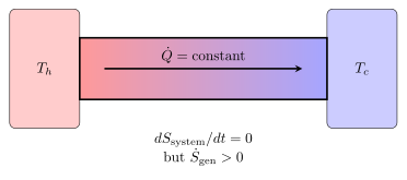
图 8:恒定 reservoirs 维持 steady heat current;profile 不变并不表示 microscopic detailed balance。
4.2 Far from equilibrium 可能出现 nonlinear instability 与 dissipative structure
当 driving 增大,linear law 可能失效,原 steady branch 可能在 threshold 失稳并分叉出新的 spatial or temporal order。结构依赖 system size、boundary condition、nonlinear kinetics 与 fluctuations;它不是第二律的例外,而是开放系统在持续 dissipation 下的组织。
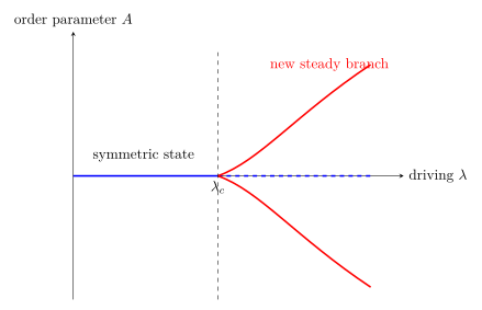
图 9:典型 supercritical bifurcation 示意;实线/虚线分别表示稳定/失稳分支,不代表所有远离平衡系统。
不能把“minimum entropy production”或“maximum entropy production”当作任意 NESS 的普遍变分原理。某些近 equilibrium、固定约束的线性系统有特定 extremum result;far-from-equilibrium branch selection 通常必须求具体动力学与稳定性。
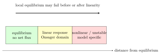
图 10:Onsager linear regime 是近 equilibrium 区域;local equilibrium 与 linearity 是不同假设,应分别审计。
Worked Example 4 — Thermostatted conductor 的 NESS entropy production
已知: 长 \(L=0.100\ \mathrm m\)、截面积 \(A=1.00\times10^{-6}\ \mathrm{m^2}\) 的均匀 conductor,\(\sigma_e=1.00\times10^5\ \mathrm{S\,m^{-1}}\),施加 \(E=10.0\ \mathrm{V\,m^{-1}}\)。恒温器保持 \(T=300\ \mathrm K\)。求 current、Joule power 与 total entropy-production rate。
系统边界: conductor 是开放能量系统;thermostat 移走全部 Joule heat。
参考系与方向: lattice 实验室系,\(\mathbf E\) 为正方向。
模型理由: Ohmic steady response,temperature uniform,忽略 contact resistance。
\[j=\sigma_eE =1.00\times10^6\ \mathrm{A\,m^{-2}}, \qquad I=jA=1.00\ \mathrm A.\]
Potential drop 为 \(\Delta V=EL=1.00\ \mathrm V\),故
\[P=I\Delta V=1.00\ \mathrm W.\]
Conductor 的 energy 与 entropy 不随时间累积,但
\[\boxed{ \dot S_{\mathrm{gen}}=\frac{P}{T} =3.33\times10^{-3}\ \mathrm{W\,K^{-1}}. }\]
检查: 同时用 \(jE(AL)\) 得 \(1.00\ \mathrm W\);断开电场时 \(I\)、\(P\)、entropy production 全部归零。稳态电流和正耗散证明该状态不是 equilibrium。
Lesson synthesis / 全课整合
Irreversible thermodynamics 的逻辑链是:
- 用 local-equilibrium cells 定义 \(T,\mu,p\) 等局域强度量;
- 对 mass、energy 与 entropy 写局域 balance;
- 把 \(\sigma_s\) 整理为共轭 flux-force products;
- near equilibrium 时线性化 \(\mathbf J=\mathbf L\mathbf X\);
- 用 second law 检查 \(\mathbf L\) 的 positive semidefinite symmetry part;
- 只有再加入 microscopic reversibility 与正确 time-reversal parity,才使用 Onsager/Onsager–Casimir reciprocity;
- 对 NESS 同时核算 system 与 reservoirs;若 driving 不小,回到具体 nonlinear dynamics 和 stability analysis。
Formula-and-decision table / 公式—决策表
| Task | Relation | Use only when | Key caution |
|---|---|---|---|
| local entropy balance | \(\partial_ts+\nabla\cdot\mathbf J_s=\sigma_s\) | continuum local fields exist | flux divergence is not production |
| heat entropy production | \(\sigma_s=\mathbf q\cdot\nabla(1/T)\) | heat conduction in local equilibrium | \(\mathbf q\) pairs with \(\nabla(1/T)\) |
| diffusion force | \(\mathbf X_a=-\nabla(\mu_a/T)\) | flux defined in stated material frame | multicomponent constraints matter |
| reaction contribution | \(\sigma_{s,r}=\mathcal R_r\mathcal A_r/T\) | affinity convention declared | rate and affinity signs must match |
| linear laws | \(\mathbf J_i=\sum_jL_{ij}\mathbf X_j\) | near equilibrium | coefficients may depend on state |
| second-law matrix test | \(\mathbf X^{\mathsf T}\mathbf L\mathbf X\ge0\) | same conjugate normalization | constrains symmetric part |
| Onsager reciprocity | \(L_{ij}=L_{ji}\) | microscopic reversibility, no odd field | not derived from second law alone |
| Onsager–Casimir | \(L_{ij}(\mathbf B)=\epsilon_i\epsilon_jL_{ji}(-\mathbf B)\) | time-reversal parity identified | reverse magnetic/rotation fields |
| NESS entropy ledger | \(\dot S_{\mathrm{gen}}=\sum \dot Q_{\mathrm{out}}/T_{\mathrm{out}}-\sum \dot Q_{\mathrm{in}}/T_{\mathrm{in}}\) | steady system; \(\dot Q_{\mathrm{in/out}}\) are nonnegative magnitudes | \(dS_{\mathrm{system}}/dt=0\) is not reversibility |
Model boundaries / 模型边界
- Local equilibrium fails when mean free path, correlation length or local relaxation time is not separated from observation scales.
- Flux definitions depend on reference velocity; changing frame reshuffles heat and diffusion fluxes and their conjugate forces.
- Onsager reciprocity requires near-equilibrium linear response and microreversibility; magnetic fields require Casimir parity factors.
- Positive entropy production constrains only admissible constitutive laws; it does not uniquely determine all coefficients.
- A global system may be far from equilibrium while each cell remains locally near equilibrium; conversely ultrafast transport may destroy local equilibrium even for a modest macroscopic difference.
- Dissipative structures require open driving and nonlinear stability analysis; a schematic pitchfork is not a universal phase diagram.
- No unrestricted extremum principle selects all far-from-equilibrium steady states.
Misconception clinic / 易错概念诊所
- “Local equilibrium 表示每个位置都没有 flux。” 错;cell 内可定义 equilibrium variables,而 cell 间梯度驱动 flux。
- “稳态时 entropy production 必须为零。” 错;NESS 中内部产生由边界 entropy export 平衡。
- “任何 gradient 都可叫 thermodynamic force。” 错;共轭配对必须从 entropy-production decomposition 确定。
- “第二律自动证明 \(L_{ij}=L_{ji}\)。” 错;第二律给 positivity,reciprocity 还用 microscopic reversibility。
- “磁场中仍总有 \(L_{ij}=L_{ji}\)。” 错;必须使用 field-reversed Onsager–Casimir relation。
- “远离平衡出现有序结构说明 entropy 减少。” 错;开放系统可在向环境输出 entropy 的同时维持内部 order,总 entropy production 仍非负。
Practice and retrieval / 练习与检索
1. 尺度分离(K01)
若 mean free path \(20\ \mathrm{nm}\)、gradient scale \(2\ \mathrm{\mu m}\),给出一个可能的 local cell size,并说明为什么。
Answer
例如 \(\ell_c=200\ \mathrm{nm}\),满足 \(20\ \mathrm{nm}\ll200\ \mathrm{nm}\ll2\ \mathrm{\mu m}\)。还需检查 local relaxation time;空间不等式本身不是充分条件。
2. Entropy balance(K01)
一个 steady control volume 每秒输出 \(0.80\ \mathrm{W\,K^{-1}}\) entropy、输入 \(0.50\ \mathrm{W\,K^{-1}}\)。内部 production 是多少?
Answer
稳态 \(0=\dot S_{\mathrm{in}}-\dot S_{\mathrm{out}}+\dot S_{\mathrm{gen}}\),所以 \(\dot S_{\mathrm{gen}}=0.30\ \mathrm{W\,K^{-1}}\)。
3. Heat-force sign(K02)
为什么 heat-conduction force 选 \(\nabla(1/T)\) 而不是 \(\nabla T\)?
Answer
Fourier heat flux 与 \(\nabla T\) 反向;选 \(\nabla(1/T)=-\nabla T/T^2\) 后 \(\mathbf q\cdot\nabla(1/T)=k\lvert\nabla T\rvert^2/T^2\ge0\),并自然给 entropy-production unit。
4. Chemical affinity(K02)
若采用正 reaction rate 表示 forward reaction,affinity 的正号应怎样选?
Answer
应选使 spontaneous forward reaction 有 \(\mathcal R\mathcal A/T\ge0\) 的 convention。若改变 reaction stoichiometric direction,rate 与 affinity 必须同时反号。
5. Positivity test(K03)
\(\mathbf L=\begin{pmatrix}2&3\\3&2\end{pmatrix}\) 能否作为 symmetric linear-response matrix?
Answer
不能作为所有 forces 下的 dissipative matrix,因为 determinant \(4-9=-5<0\),存在方向使 \(\mathbf X^{\mathsf T}\mathbf L\mathbf X<0\)。
6. Reciprocity 的额外前提(K03)
列出 second law positivity 之外,应用简单 Onsager reciprocity 的两个前提。
Answer
Near-equilibrium linear response;microscopic reversibility 且没有未反转的 time-reversal-odd field。还必须使用真正共轭的 force/flux normalization。
7. Magnetic field(K03)
为什么测 \(L_{12}(+\mathbf B)\) 时通常应与 \(L_{21}(-\mathbf B)\) 比较?
Answer
Time reversal 会反转 magnetic field;Onsager–Casimir relation 比较的是 time-reversed experiment,并附带 variables 的 parity factors。
8. NESS 判断(K04)
温度 profile 恒定、heat current 非零。该状态是 equilibrium 吗?
Answer
不是。它是由 reservoirs 维持的 NESS;宏观 profile stationary,但存在 flux、broken detailed balance 与 positive entropy production。
9. Reservoir ledger(K04)
\(10.0\ \mathrm W\) 从 \(500\ \mathrm K\) reservoir 流到 \(250\ \mathrm K\) reservoir。求 total entropy-production rate。
Answer
\(\dot S_{\mathrm{gen}}=10(1/250-1/500)=2.00\times10^{-2}\ \mathrm{W\,K^{-1}}\)。
10. Far-from-equilibrium boundary(K04)
为什么 observation 到 \(\sigma_s\) 较大不能单独决定 system 会选择哪个 nonlinear steady branch?
Answer
Second law 只要求 admissible evolution 的 total production 非负;branch selection 还取决于 nonlinear dynamics、boundary conditions、stability、noise 与 initial conditions。不存在无条件的通用最大或最小 entropy-production selector。
Exit ticket / 课末检验
- 对同时有 heat 与 solute flux 的 system,写出 local entropy balance、两个 force-flux products,以及验证 \(2\times2\) coefficient matrix 的步骤。
- 用一句话分别定义 equilibrium、near-equilibrium linear response 和 NESS,再说明 far-from-equilibrium bifurcation 为什么不超出第二律。
References and source notes / 参考资料与来源说明
- MIT OCW 5.72, Non-equilibrium Thermodynamics — response、relaxation、Onsager regression 与 linear-response framework。
- MIT OCW 2.43, Lecture 21 — Introduction to Nonequilibrium Theory; Onsager Reciprocity and Maximum Entropy Production — near-equilibrium force–flux linearization、Onsager reciprocity、steady heat conduction 与 nonlinear boundary。
- Lars Onsager, Reciprocal Relations in Irreversible Processes I, Physical Review 37, 405 (1931) — 原始 reciprocity、entropy production 与 microscopic fluctuation argument。
- Lars Onsager, Reciprocal Relations in Irreversible Processes II, Physical Review 38, 2265 (1931) — coupled heat/electric/diffusion transport 与 magnetic-field reversal。
- IUPAC Gold Book — Microscopic Reversibility at Equilibrium — equilibrium microscopic reversibility 的官方术语边界。
- Ilya Prigogine — Nobel Lecture — far-from-equilibrium bifurcations、dissipative structures、global boundary dependence 与 nonlinear branch。
- 1977 Nobel Prize in Chemistry — Official Press Release — near-equilibrium Onsager domain 与 Prigogine far-from-equilibrium contribution 的历史范围。
以上直接来源均于 2026-08-25 实际打开并核对到具体 lecture notes、原始论文或官方术语/诺奖页面。正文没有把任何 source 的 extremum statement 扩张为普遍定律;全部图示由本文方程和模型原创。
Source-to-content map
| Source | Used for | Knowledge ID / Section | Model boundary or convention |
|---|---|---|---|
| MIT 5.72 Chapter 2 | response, relaxation and nonequilibrium framework | K01–K03 | graduate scope compressed to local linear theory |
| MIT 2.43 Lecture 21 | linear force–flux laws and heat-conduction NESS | K02–K04 | near/far boundary stated explicitly |
| Onsager 1931 I | reciprocity and entropy-production structure | K03 | microreversibility, near equilibrium |
| Onsager 1931 II | coupled transport and field reversal | K03 | magnetic-field comparison retained |
| IUPAC Gold Book | microscopic reversibility definition | K03 | equilibrium terminology |
| Prigogine Nobel lecture | nonlinear instability and dissipative structure | K04 | model-specific far-from-equilibrium branches |
| Nobel official press release | historical domain distinction | K03, K04 | not used as a derivation source |
复习与拓展
- Electromagnetism 将提供 \(\mathbf E\)、current 与 magnetic-field reversal 的具体实现。
- Fluid dynamics and plasma physics 将把 entropy production、viscosity、heat flux 与 multicomponent diffusion 写成 tensor transport。
- Linear response/Kubo theory 会把 \(L_{ij}\) 表示为 equilibrium correlation functions。
- Stochastic thermodynamics 将在单条 trajectory 上定义 work、heat 与 entropy production fluctuation relations。