电感与 RL 电路 · Inductance and RL Circuits

Learning objectives / 学习目标

完成本课后，你应能：

用 flux linkage 定义 self-inductance 与 mutual inductance，并正确使用点标记或明确电流/电压参考方向；
从功率 $$p=vi$$ 推导 $$U_B=LI^2/2$$ ，并连接到真空场能密度 $u_B=B^2/(2\mu_0)$ ；
求解 RL 接通与断开暂态，解释 $\tau=L/R$ 、电流连续性和初末极限；
推导理想变压器的电压比、电流比与反射阻抗，并指出漏磁、绕组电阻、磁化电流和铁损边界；
用 $\mathcal E_{\rm back}=k_e\omega$ 建立电机端口功率账本，解释堵转电流与负载变化。

Prerequisites / 先修知识

Faraday's and Lenz's Laws：flux linkage 与 Lenz 符号。
Motional EMF and Electric Generators：机械—电能转换。
Kirchhoff loop rule、一阶线性微分方程、指数函数与时间常数。
长螺线管近似 $B=\mu_0NI/\ell$ 。

Scope and conventions / 范围与约定

采用 passive sign convention：电流进入标为正电压的端子时，元件吸收功率 $$p=vi$$ 。
理想线性电感满足 $\lambda=LI$ ；若磁芯非线性或有磁滞， $$L$$ 可随工作点和历史变化。
互感符号由绕组方向、参考电流方向与 dot convention 决定； $$M$$ 的大小非负，互感项的代数号另行判断。
RL 采用 lumped、恒定 $$R,L$$ ；开关电弧、寄生电容与传输线效应暂不讨论。
理想变压器假设同一磁通链过所有匝、无损耗、无漏磁、磁化电流可忽略；真实器件需等效电路修正。
TikZ 均为 schematic / not to scale。

Notation and modeling contract / 符号与建模契约

Symbol	Meaning	SI unit
$\lambda=N\Phi_B$	flux linkage	Wb-turn
$L=d\lambda/dI$	differential self-inductance	H
$$M$$	mutual inductance magnitude	H
$k=M/\sqrt{L_1L_2}$	coupling coefficient	dimensionless
$$U_B,u_B$$	magnetic energy and energy density	J, $\mathrm{J\,m^{-3}}$
$\tau=L/R$	RL time constant	s
$$N_p,N_s$$	primary and secondary turns	—
$k_e\omega$	rotational back emf in a linear motor model	V

Knowledge 1 — Self-inductance and mutual inductance / 自感与互感

Knowledge ID: P04-U08-L03-K01

电流产生磁场，磁场又给原回路造成 flux linkage。在线性、几何固定的单回路中

$\lambda=N\Phi_B=LI, \qquad \mathcal E_L=-\frac{d\lambda}{dt}=-L\frac{dI}{dt}.$

更一般地，瞬时 differential inductance 为 $L_d=d\lambda/dI$ ；只有 $\lambda$ – $$I$$ 直线通过原点时，常数 $L=\lambda/I$ 与 $$L_d$$ 相同。

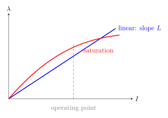
Inductance and RL Circuits — Knowledge 1 — Self-inductance and mutual inductance / 自感与互感（图 1） — 图 1Knowledge 1 — Self-inductance and mutual inductance / 自感与互感

图 1 区分常数电感与非线性 differential inductance；后者不能直接套用 $$LI^2/2$$ 。

两个回路耦合时，回路 1 的电流在回路 2 中产生

$\lambda_{21}=M_{21}I_1, \qquad \mathcal E_2=-M_{21}\frac{dI_1}{dt}.$

在互易、静止、线性介质中 $M_{12}=M_{21}=M$ 。能量正定给

$M^2\le L_1L_2, \qquad 0\le k=\frac{M}{\sqrt{L_1L_2}}\le1.$

点标记规则：若参考电流同时进入两个 dot terminals，互感电压项取同号；若一进一点而另一离开点，则取反号。

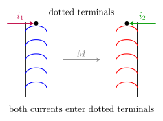
Inductance and RL Circuits — Knowledge 1 — Self-inductance and mutual inductance / 自感与互感（图 2） — 图 2Knowledge 1 — Self-inductance and mutual inductance / 自感与互感

图 2 将互感符号与参考方向绑定；只说“同名端”而不画电流方向仍不够。

Knowledge 2 — Energy stored in magnetic fields / 磁场储能

Knowledge ID: P04-U08-L03-K02

理想电感端口电压按 passive convention 为 $v_L=L\,dI/dt$ 。外电路向电感输入功率

$p_L=v_LI=LI\frac{dI}{dt}.$

从 $$0$$ 建立到 $$I$$ ：

$U_B=\int_0^t p_Ldt =\int_0^I LI'\,dI' =\frac12LI^2.$

能量储存在磁场及其介质响应中，不是“藏在导线里”。真空或线性介质中

$u_B=\frac12\mathbf B\cdot\mathbf H,$

真空即 $u_B=B^2/(2\mu_0)$ 。非线性无磁滞、可逆材料应写 $u_B=\int_0^{\mathbf B}\mathbf H\cdot d\mathbf B'$ ；有磁滞时一周回线面积对应耗散，不能用单值状态函数覆盖全过程。

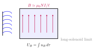
Inductance and RL Circuits — Knowledge 2 — Energy stored in magnetic fields / 磁场储能（图 3） — 图 3Knowledge 2 — Energy stored in magnetic fields / 磁场储能

图 3 把 lumped energy 与 field energy 连接：用长螺线管场积分可复得 $L=\mu_0N^2A/\ell$ 。

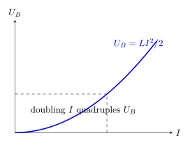
Inductance and RL Circuits — Knowledge 2 — Energy stored in magnetic fields / 磁场储能（图 4） — 图 4Knowledge 2 — Energy stored in magnetic fields / 磁场储能

图 4 表明线性电感能量随 $$I^2$$ ；电流方向反转不改变储能，但磁场方向反转。

Knowledge 3 — RL growth and decay / RL 电路增长与衰减

Knowledge ID: P04-U08-L03-K03

直流源 $\mathcal E$ 接入串联 $$R,L$$ 后，回路方程为

$L\frac{dI}{dt}+RI=\mathcal E.$

若 $$I(0)=0$$ ，解为

$I(t)=\frac{\mathcal E}{R}\left(1-e^{-t/\tau}\right), \qquad \tau=\frac{L}{R}.$

端电压为 $v_L=\mathcal Ee^{-t/\tau}$ 与 $v_R=\mathcal E(1-e^{-t/\tau})$ 。初始电感承担全部源电压，长期后理想电感相当于导线；“相当于导线”仅指稳定直流端口，不意味着其场能为零。

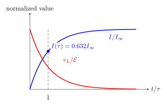
Inductance and RL Circuits — Knowledge 3 — RL growth and decay / RL 电路增长与衰减（图 5） — 图 5Knowledge 3 — RL growth and decay / RL 电路增长与衰减

图 5 显示同一指数在电流增长与电感电压衰减中的互补关系。

断开电源但给电流提供 $$R$$ 闭合路径，

$L\frac{dI}{dt}+RI=0, \qquad I(t)=I_0e^{-t/\tau}.$

理想电感电流不能瞬间跳变：若有限 $$L$$ 下 $\Delta I$ 在零时间发生， $L\,dI/dt$ 需无限电压。真实开关若不给安全路径，寄生电容、空气击穿或电弧会承受高压。

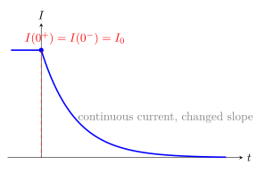
Inductance and RL Circuits — Knowledge 3 — RL growth and decay / RL 电路增长与衰减（图 6） — 图 6Knowledge 3 — RL growth and decay / RL 电路增长与衰减

图 6 区分连续性与“保持不变”：开关后电流值连续，但导数立即改变。

Knowledge 4 — Transformers and coupled circuits / 变压器与耦合电路

Knowledge ID: P04-U08-L03-K04

理想变压器两绕组共享每匝磁通 $\Phi(t)$ ：

$v_p=-N_p\frac{d\Phi}{dt}, \qquad v_s=-N_s\frac{d\Phi}{dt}.$

上式中的小写 $$v_p,v_s$$ 是按各自绕组参考极性定义的瞬时有符号电压。为避免与全课 passive sign convention 混淆，本小节以下用大写 $$V_p,V_s,I_p,I_s$$ 专指正的 RMS 幅值。于是幅值变比为

$\frac{V_s}{V_p}=\frac{N_s}{N_p}=n.$

若两个端口电流都按 passive sign convention 定义为流入各自正端，则无损器件的有符号端口功率满足 $$v_pi_p+v_si_s=0$$ 。同一结论用正的 RMS 幅值写成

$V_pI_p=V_sI_s, \qquad \frac{I_s}{I_p}=\frac{N_p}{N_s}=\frac{1}{n}.$

因此负载阻抗反射到原边：

$Z_{\rm in}=\left(\frac{N_p}{N_s}\right)^2Z_L.$

升压不会免费放大功率；它以电流下降为代价。

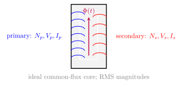
Inductance and RL Circuits — Knowledge 4 — Transformers and coupled circuits / 变压器与耦合电路（图 7） — 图 7Knowledge 4 — Transformers and coupled circuits / 变压器与耦合电路

图 7 是理想 common-flux 模型；真实变压器还需串联绕组电阻/漏感、并联磁化电感与铁损支路。

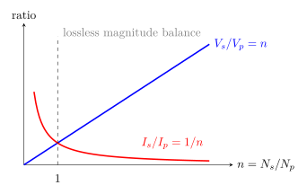
Inductance and RL Circuits — Knowledge 4 — Transformers and coupled circuits / 变压器与耦合电路（图 8） — 图 8Knowledge 4 — Transformers and coupled circuits / 变压器与耦合电路

图 8 把升压与降流画在同一 turns-ratio 轴上；蓝、红两条曲线都表示正的 RMS 幅值比，而不是同时流入两端口的有符号电流比。

Knowledge 5 — Back emf in motors and generators / 电动机与发电机中的反电动势

Knowledge ID: P04-U08-L03-K05

旋转电机的线圈同时是发电机。在线性简化模型中

$\mathcal E_{\rm back}=k_e\omega, \qquad V_s=IR+L\frac{dI}{dt}+\mathcal E_{\rm back}.$

稳定转速时 $$dI/dt=0$$ ：

$I=\frac{V_s-k_e\omega}{R}.$

堵转 $\omega=0$ 时 back emf 为零，电流约 $$V_s/R$$ ，可能非常大；转速上升后 back emf 增大，电流下降。负载突然增大使电机减速，back emf 降低，电流与电磁转矩随之增加。

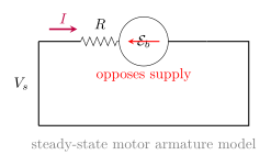
Inductance and RL Circuits — Knowledge 5 — Back emf in motors and generators / 电动机与发电机中的反电动势（图 9） — 图 9Knowledge 5 — Back emf in motors and generators / 电动机与发电机中的反电动势

图 9 的 back emf 极性反对源电压。机电功率 $P_{\rm conv}=\mathcal E_{\rm back}I$ ；铜耗 $$I^2R$$ ，源功率 $$V_sI$$ ，忽略机械损耗时三者满足守恒。

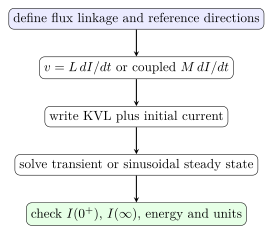
Inductance and RL Circuits — Knowledge 5 — Back emf in motors and generators / 电动机与发电机中的反电动势（图 10） — 图 10Knowledge 5 — Back emf in motors and generators / 电动机与发电机中的反电动势

图 10 是电感问题的统一决策链；初值与参考方向缺一不可。

Worked Examples / 完整例题

Worked Example 1 — Long-solenoid inductance and energy / 长螺线管电感与储能

已知条件： $$N=800$$ ， $A=4.00\times10^{-4}\ \mathrm{m^2}$ ，长度 $\ell=0.400\ \mathrm m$ ，空气芯，电流 $I=2.00\ \mathrm A$ 。
研究对象与边界： 整个螺线管及其磁场。
参考系与正方向： 实验室系；绕组正方向按右手规则定义正磁通。
模型及理由： $\ell$ 远大于横向尺度，忽略边缘场，线性真空。

$L=\frac{\mu_0N^2A}{\ell} =\frac{(4\pi\times10^{-7})(800)^2(4.00\times10^{-4})}{0.400} =8.04\times10^{-4}\ \mathrm H.$

$U_B=\frac12LI^2 =\frac12(8.04\times10^{-4})(2.00)^2 =1.61\times10^{-3}\ \mathrm J.$

结论： $L=0.804\ \mathrm{mH}$ ， $U_B=1.61\ \mathrm{mJ}$ 。
检查： $$L$$ 与 $$I$$ 无关只因采用线性空气芯；能量随 $$I^2$$ 。用 $B=\mu_0NI/\ell$ 和 $u_B=B^2/(2\mu_0)$ 积分会得到同一结果。

Worked Example 2 — RL turn-on at two time constants / 两个时间常数后的 RL 接通

已知条件： $\mathcal E=12.0\ \mathrm V$ ， $R=6.00\ \Omega$ ， $L=0.300\ \mathrm H$ ， $$I(0)=0$$ ；求 $t=0.100\ \mathrm s$ 的 $$I,v_R,v_L$$ 。
研究对象与边界： 串联源、 $$R$$ 、 $$L$$ 整回路。
参考系与正方向： 电流从源正端流出；元件用 passive sign convention。
模型及理由： 理想恒压源与常数线性元件。

$\tau=\frac{L}{R}=0.0500\ \mathrm s, \qquad t/\tau=2.00.$

$I=\frac{12.0}{6.00}(1-e^{-2})=1.73\ \mathrm A.$

$v_L=12.0e^{-2}=1.62\ \mathrm V, \qquad v_R=RI=10.4\ \mathrm V.$

结论： $I=1.73\ \mathrm A$ ， $v_R=10.4\ \mathrm V$ ， $v_L=1.62\ \mathrm V$ 。
检查： $v_R+v_L=12.0\ \mathrm V$ （舍入内）； $I<\mathcal E/R=2.00\ \mathrm A$ 。初始时 $$I=0$$ 、末态 $$v_L=0$$ 的极限都正确。

Worked Example 3 — Ideal transformer with load / 带负载理想变压器

已知条件： $$N_p=500$$ ， $$N_s=100$$ ， $V_p=230\ \mathrm{V_{rms}}$ ，次级接 $R_L=9.20\ \Omega$ 。
研究对象与边界： 理想变压器加次级电阻负载。
参考系与正方向： RMS 相量幅值；功率流从原边到次边。
模型及理由： common flux、无损、忽略磁化电流。

$V_s=V_p\frac{N_s}{N_p}=230\frac{100}{500}=46.0\ \mathrm V.$

$I_s=\frac{V_s}{R_L}=5.00\ \mathrm A, \qquad I_p=I_s\frac{N_s}{N_p}=1.00\ \mathrm A.$

$P_p=V_pI_p=230\ \mathrm W, \qquad P_s=V_sI_s=230\ \mathrm W.$

结论： $V_s=46.0\ \mathrm V$ ， $I_s=5.00\ \mathrm A$ ， $I_p=1.00\ \mathrm A$ 。
检查： 降压比 $$1/5$$ 对应升流比 $$5$$ ，功率守恒。原边看见 $Z_{\rm in}=(500/100)^2(9.20)=230\ \Omega$ ，故 $230/230=1.00\ \mathrm A$ ，一致。

Worked Example 4 — Motor back-emf power balance / 电机反电动势功率账本

已知条件： $V_s=48.0\ \mathrm V$ ，绕组 $R=0.400\ \Omega$ ， $k_e=0.0500\ \mathrm{V\,s\,rad^{-1}}$ ，稳定转速 $\omega=800\ \mathrm{rad\,s^{-1}}$ 。
研究对象与边界： 电机电端口与理想机电转换端口；忽略机械损耗。
参考系与正方向： 电流进入电机正端；正转速产生反对电源的 emf。
模型及理由： 稳态 $$dI/dt=0$$ 、线性 $\mathcal E_b=k_e\omega$ 。

$\mathcal E_b=(0.0500)(800)=40.0\ \mathrm V,$

$I=\frac{48.0-40.0}{0.400}=20.0\ \mathrm A.$

$P_{\rm source}=V_sI=960\ \mathrm W, \quad P_{\rm copper}=I^2R=160\ \mathrm W, \quad P_{\rm conv}=\mathcal E_bI=800\ \mathrm W.$

结论： back emf $40.0\ \mathrm V$ 、电流 $20.0\ \mathrm A$ 、理想机械转换功率 $800\ \mathrm W$ 。
检查： $960=160+800\ \mathrm W$ 。若堵转，理想电流会升至 $48.0/0.400=120\ \mathrm A$ ，说明需要限流与热保护。

Lesson synthesis / 课程综合

电感是“磁通链对电流的响应”，不是简单线圈外形标签。其反馈把五个表象统一起来：

自感用 $-d\lambda/dt$ 阻碍自身电流变化；
外源做功建立 $$LI^2/2$$ 的磁场能；
与电阻组合产生 $$L/R$$ 时间尺度；
互感通过共同磁通转移电压与电流；
旋转电机的 back emf 把转速反馈到电流和转矩。

Formula-and-decision table / 公式与决策表

Situation	Formula	Conditions / limits
线性自感	$\lambda=LI$ , $v_L=L\,dI/dt$	passive sign convention；几何与材料线性
互感	$\lvert v_2\rvert=M\lvert dI_1/dt\rvert$	代数号由点标记与参考方向决定
线性储能	$$U_B=LI^2/2$$	$$L$$ 常数、可逆
真空场能密度	$u_B=B^2/(2\mu_0)$	真空；一般线性介质用 $\mathbf B\cdot\mathbf H/2$
RL 接通	$I=(\mathcal E/R)(1-e^{-tR/L})$	$$I(0)=0$$ 、恒压源
RL 衰减	$I=I_0e^{-tR/L}$	有闭合耗散路径
理想变压器	$$V_s/V_p=N_s/N_p$$ ， $$V_pI_p=V_sI_s$$	正的 RMS 幅值；若两端口均用 passive sign，则 $$v_pi_p+v_si_s=0$$
反射阻抗	$Z_{\rm in}=(N_p/N_s)^2Z_L$	理想变压器
电机稳态	$I=(V_s-k_e\omega)/R$	线性 back emf、 $$dI/dt=0$$

Model boundaries / 模型边界

铁芯接近饱和或存在磁滞时， $$L$$ 不是固定常数， $$U=LI^2/2$$ 也可能失效。
电感电流连续性假设有限电压；电弧或寄生电容可允许快速但仍非理想的变化。
理想变压器不传递 DC 稳态： $d\Phi/dt=0$ 时次级无持续感应电压；直流接原边还可能导致过流/饱和。
back emf 与 self-inductive emf 不是同一项：前者主要来自转动改变磁通，后者来自电流变化。
lumped RL 忽略空间传播与辐射；高频时必须用分布参数与 Maxwell 场。

Misconception clinic / 误区诊所

“电感永远反对电流。” 它反对电流的变化；断电时会维持原方向电流。
“稳态直流下电感没有能量。” 理想电感端电压为零，但若 $I\ne0$ ，仍有 $$LI^2/2$$ 场能。
“升压变压器也升高电流。” 理想功率守恒下，电压升高伴随电流降低。
“ $$M$$ 可任意大。” 被动线性耦合满足 $M^2\le L_1L_2$ ；否则能量二次型会失去正定性。
“电机慢下来就少用电。” back emf 下降会使电流增大；重载低速可能更易过热。

Practice and retrieval / 练习与检索

[P04-U08-L03-K01] 某线圈在 $I=2.00\ \mathrm A$ 时 flux linkage 为 $0.120\ \mathrm{Wb\!\cdot turn}$ ，线性。求 $$L$$ 。

Answer

$L=\lambda/I=0.120/2.00=0.0600\ \mathrm H$ 。

[P04-U08-L03-K01] $L_1=4.00\ \mathrm H$ 、 $L_2=9.00\ \mathrm H$ ，被动互易耦合的 $$M$$ 最大多少？

Answer

$M\le\sqrt{L_1L_2}=\sqrt{36.0}=6.00\ \mathrm H$ ；等号对应理想完全耦合 $$k=1$$ 。

[P04-U08-L03-K02] $L=0.500\ \mathrm H$ 中电流从 $2.00\ \mathrm A$ 增到 $4.00\ \mathrm A$ ，储能增加多少？

Answer

$\Delta U=\tfrac12L(4.00^2-2.00^2)=3.00\ \mathrm J$ 。

[P04-U08-L03-K02] 真空中 $B=0.200\ \mathrm T$ ，求能量密度。

Answer

$u_B=B^2/(2\mu_0)=0.0400/[2(4\pi\times10^{-7})]=1.59\times10^4\ \mathrm{J\,m^{-3}}$ 。

[P04-U08-L03-K03] $L=0.240\ \mathrm H$ 、 $R=12.0\ \Omega$ ，求时间常数与衰减到初值 $$1/e$$ 的时间。

Answer

$\tau=L/R=0.0200\ \mathrm s$ ；衰减到 $$I_0/e$$ 正好需要一个时间常数，即 $20.0\ \mathrm{ms}$ 。

[P04-U08-L03-K03] RL 接通后一个时间常数，电流达到末值的多少？

Answer

$1-e^{-1}=0.632$ ，即 $63.2\%$ ；电感电压剩 $e^{-1}=36.8\%$ 。

[P04-U08-L03-K04] 理想变压器 $$N_p:N_s=10:1$$ ，次级 $12.0\ \mathrm V$ 、 $3.00\ \mathrm A$ 。求原边电压与电流。

Answer

$V_p=120\ \mathrm V$ ， $I_p=0.300\ \mathrm A$ ；两侧视在功率均为 $36.0\ \mathrm W$ 。

[P04-U08-L03-K04] $8.00\ \Omega$ 负载经 $$N_p/N_s=5.00$$ 的理想变压器反射到原边，求输入阻抗。

Answer

$Z_{\rm in}=5.00^2(8.00)=200\ \Omega$ 。

[P04-U08-L03-K05] $24.0\ \mathrm V$ 电机绕组 $R=0.600\ \Omega$ ，正常 back emf $18.0\ \mathrm V$ 。求电流与铜耗。

Answer

$I=(24.0-18.0)/0.600=10.0\ \mathrm A$ ； $P_R=I^2R=60.0\ \mathrm W$ 。

[P04-U08-L03-K05] 同一电机堵转时为什么危险？用上一题数据估算堵转电流。

Answer

堵转时 $\omega=0$ ，back emf 近零， $I\approx24.0/0.600=40.0\ \mathrm A$ ；铜耗为 $960\ \mathrm W$ ，是正常铜耗的 16 倍。

Exit ticket / 离堂检核

给出一个统一能量说明，连接 $v=L\,dI/dt$ 、 $$U=LI^2/2$$ 、RL 电流连续性与断开电弧风险。
对一个给定 turns ratio 的变压器，同时预测电压比、电流比和反射阻抗；用功率守恒检查三者是否一致。

References and source notes / 参考资料与来源说明

以下直接来源均于 2026-08-28 实际打开核验；本文采用统一 passive sign convention，来源若使用 emf 负号则在正文中转换为端口电压约定。

Source-to-content map

Source	Used for	Knowledge ID / Section	Model boundary or convention
OpenStax §14.1	mutual inductance and reciprocity	P04-U08-L03-K01	fixed linear coils
OpenStax §14.2	self-inductance and solenoid result	P04-U08-L03-K01	long-solenoid approximation
OpenStax §14.3	$$LI^2/2$$ and field energy	P04-U08-L03-K02	linear material
OpenStax §14.4	growth, decay and time constant	P04-U08-L03-K03	constant lumped $$R,L$$
OpenStax §15.6	ideal turns ratios and power	P04-U08-L03-K04	common flux and negligible losses
MIT 8.02T Ch. 11	inductance, magnetic energy, RL problem-solving	P04-U08-L03-K01, P04-U08-L03-K03	undergraduate lumped models
Feynman Vol. II Ch. 17	energy analogy, mutual bound and magnetic field energy	P04-U08-L03-K01, P04-U08-L03-K02	finite conductors and vanishing boundary fields
OpenStax §13.6	motor back emf and stall behavior	P04-U08-L03-K05	linear rotational emf model

复习与拓展

Sinusoidal Steady State 将把 $v=L\,di/dt$ 转成 $Z_L=i\omega L$ 。
RLC Circuits and Resonance 将加入电容并研究能量交换与共振。
AC Power and Transmission 将继续理想变压器、功率因数与输电损耗。