
Learning objectives / 学习目标
学完本课后,你应能:
- 分别计算 collecting area、diffraction-limited angular resolution 和 background-limited sensitivity,解释“大口径”改善的量并不完全相同;
- 依据 wavelength、seeing、thermal background、maintenance、field of view 与 cost 比较 ground/space observing,而不是宣称某平台绝对更优;
- 把 imaging、photometry、spectroscopy、polarimetry 视为不同的数据压缩与编码方式,写出 instrument response 和 calibration 的作用;
- 用 visibility 与 Fourier sampling 解释 radio aperture synthesis,区分 angular resolution、field of view 与 largest recoverable scale;
- 定义 selection function、completeness、reliability/purity,设计 injection–recovery test 并识别 flux limit、crowding 和 calibration bias。
Prerequisites / 先修知识
- Light, Spectra, and Distance 的 flux density、magnitude、spectral line 与 extinction;
- 单缝/圆孔 diffraction、two-wave interference、Fourier transform 的定性意义;
- photon counting、Poisson variance、Gaussian read noise 与 signal-to-noise ratio;
- 坐标、pixel scale、convolution 与函数采样。
Scope and conventions / 范围与约定
- \(D\) 指 circular entrance pupil diameter;中央遮挡、segmentation 与 aberration 会改变 point-spread function(PSF)。
- Rayleigh criterion \(1.22\lambda/D\) 是均匀圆孔的一个分辨约定,不是所有成像算法的硬边界;seeing、sampling 与 signal-to-noise 也决定实际可分辨性。
- Sensitivity 必须说明 source morphology、bandwidth、integration time、background、detection statistic 与 threshold;“limiting magnitude”不是仪器单一常数。
- Interferometer 的 \(B_{\max}\) 主要控制最细 angular scale,\(B_{\min}\) 控制 large-scale response,单天线 primary beam 控制 field of view;三者不可混为一个 aperture。
- Calibration 是估计 measurement operator 的过程;deconvolution 不能恢复数据从未采样的所有 modes。
Notation and modeling contract / 符号与建模契约
| Symbol | Meaning | SI / convention |
|---|---|---|
| \(D,A\) | aperture diameter and collecting area | m, \(\mathrm{m^2}\) |
| \(\lambda\) | observed wavelength | m |
| \(\theta_{\mathrm{diff}}\) | diffraction angular scale | rad |
| \(\eta\) | end-to-end throughput or quantum efficiency factor | 1 |
| \(S,B\) | source and background detected counts | electron or count |
| \(D_{\mathrm{dark}}\) | accumulated dark electrons per pixel in one exposure | electron |
| \(\sigma_{\mathrm{read}}\) | RMS read noise per pixel per read | electron |
| \(n_{\mathrm{pix}},N_{\mathrm{read}}\) | extraction pixels and number of reads | 1 |
| \(R\) | spectral resolving power \(\lambda/\Delta\lambda\) | 1 |
| \(B_{\max},B_{\min}\) | longest and shortest projected baselines | m |
| \(V(u,v)\) | complex visibility | convention-dependent |
| \(C(x)\) | completeness at true property \(x\) | probability |
Count 与 electron 可视具体 detector conversion gain 而不同;方程中必须使用同一统计单位。
1. Light gathering, angular resolution, and sensitivity / 集光、角分辨率与灵敏度
Knowledge ID: P12-U01-L03-K01
理想无遮挡圆孔的 collecting area 为:
\[A=\frac{\pi D^2}{4}.\]
在 flux 和 throughput 固定时,source photon rate 近似随 \(D^2\) 增加。圆孔 diffraction 的 Rayleigh angular scale 是:
\[\theta_{\mathrm{diff}}\simeq1.22\frac{\lambda}{D}.\]
因此大 \(D\) 同时“收更多光”并减小理想 PSF,但 sensitivity 还取决于 sky/telescope background、bandwidth、exposure、detector noise、PSF footprint 与 confusion。一个常用 counting model 是:
\[\mathrm{SNR}=\frac{S}{\sqrt{S+B+n_{\mathrm{pix}}\left(D_{\mathrm{dark}}+N_{\mathrm{read}}\sigma_{\mathrm{read}}^2\right)}}.\]
这里 \(S\) 与 \(B\) 是 extraction aperture 内同一次曝光的总期望 counts,\(D_{\mathrm{dark}}\) 是每像素在该曝光累计的 dark electrons;read-noise variance 按 \(N_{\mathrm{read}}\) 次读出与 \(n_{\mathrm{pix}}\) 个 pixels 累加。单次读出即 \(N_{\mathrm{read}}=1\)。若 background dominated,SNR 通常随 \(\sqrt t\) 增长;若系统误差或 confusion 主导,延长曝光不会无限改善。
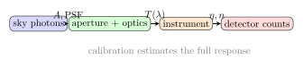
图 1 展示 telescope–instrument–detector 是一个串联系统;不能把 detector counts 直接等同于 source flux。
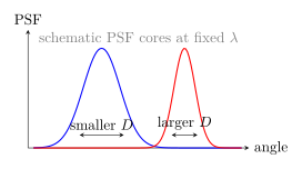
图 2 用示意 PSF 比较口径;真实 Airy pattern 有 rings,宽度并非 Gaussian,但 \(\lambda/D\) scaling 保留。
2. Ground- and space-based observing / 地基与空间观测
Knowledge ID: P12-U01-L03-K02
Ground facilities 可建更大口径、维护升级方便、单位成本通常较低;但 atmosphere 带来 transmission windows、absorption bands、sky emission、weather 与 seeing。Adaptive optics 通过测量 wavefront distortion 并实时校正,可在有限 field/wavelength/reference-source 条件下接近 diffraction limit,却不消除所有大气背景或吸收。
Space observatories 位于大气之上,可进入大部分 UV、X-ray、gamma-ray 和被地面水汽遮挡的 infrared bands,并获得稳定 PSF;但 launch mass/volume、thermal design、radiation damage、telemetry、serviceability 和 cost 形成新的边界。空间望远镜也受 diffraction、stray light、detector persistence 与 calibration drift 影响。
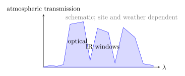
图 3 是大气窗口示意而非定量 transmission curve;它说明“地面/空间”选择首先是 wavelength-dependent trade-off。
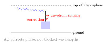
图 4 区分 adaptive optics 的 wavefront correction 与 space access;AO 不能让被大气强吸收的 band 重新透过。
3. Imaging, photometry, spectroscopy, and polarimetry / 成像、测光、光谱与偏振测量
Knowledge ID: P12-U01-L03-K03
四种常见模式回答不同问题:
- Imaging: 保留二维 sky position,通常在有限 band 内积分;
- Photometry: 通过 aperture/PSF fit 浓缩为 calibrated flux 或 magnitude,适合 time series 和 colors;
- Spectroscopy: 把光分散到 wavelength bins,分辨本领 \(R=\lambda/\Delta\lambda\);每 bin 光子更少;
- Polarimetry: 测 Stokes parameters \((I,Q,U,V)\),探测 scattering geometry、magnetic fields 与 aligned dust,但易受 instrumental polarization 影响。
可把整个观测写成 measurement operator:
\[\mathbf d=\mathbf R(\boldsymbol\gamma)\mathbf s+\mathbf n,\]
\(\mathbf s\) 是真实 sky brightness/spectrum/polarization,\(\mathbf R\) 包含 PSF、throughput、dispersion、pixel response 和 pointing,\(\boldsymbol\gamma\) 是 calibration parameters。Reduction 不是删除噪声,而是估计/边缘化 \(\boldsymbol\gamma\) 并保留 covariance。
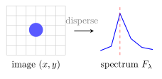
图 5 显示 spectroscopy 用 spatial information 换取 wavelength information(普通长缝情况下);integral-field spectroscopy 可同时采样三维 data cube,但成本与数据量更高。
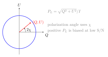
图 6 是线偏振的 \(Q\)–\(U\) 平面;\(P_L\) 为正定量,低信噪比下直接取平方根会有正偏差。
4. Radio interferometry and aperture synthesis / 射电干涉与孔径合成
Knowledge ID: P12-U01-L03-K04
两天线接收同一窄带天空场的相关信号,得到 complex visibility。对 small field、近似平面波与适当坐标,van Cittert–Zernike relation 的简化形式是:
\[V(u,v)=\iint I(l,m)e^{-2\pi i(ul+vm)}\,dl\,dm.\]
每条 projected baseline \(\mathbf B/\lambda\) 采样一个 Fourier-plane point;Earth rotation 与多天线 pairs 填充 \(uv\) coverage。有限采样的 inverse transform 得到 true sky 与 synthesized beam(dirty beam)的 convolution,再用带假设的 deconvolution 估计图像。
近似尺度:
\[\theta_{\mathrm{res}}\sim\frac{\lambda}{B_{\max}},\]
而大于约 \(\lambda/B_{\min}\) 数量级的平滑结构会被空间滤除。Long baseline 提高 fine-detail resolution,但不自动增加 total collecting area 或 surface-brightness sensitivity;缺少 short spacings 的 diffuse flux 不能凭 deconvolution 完全恢复。
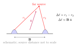
图 7 把 source 移离 baseline 的垂直平分线,因此两条路径不等长;远场近似下 geometric delay 为 \(\tau_g=\Delta\ell/c\simeq\mathbf B\cdot\hat{\mathbf s}/c\)(符号随 baseline orientation 定义)。实际 correlator 还要补偿 clock、atmosphere 与 electronics phase。
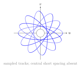
图 8 表示 Earth-rotation synthesis 的 \(uv\) tracks。中心空洞对应缺少 short baselines,会损失大尺度结构;图不是某一具体阵列的比例图。
5. Selection effects, calibration, and survey completeness / 选择效应、校准与巡天完备性
Knowledge ID: P12-U01-L03-K05
Catalog 不是“天空中所有源”的无偏列表。Selection function 是真参数到被纳入样本概率的映射:
\[C(x,\mathbf r)=P(\mathrm{detected\ and\ selected}\mid x,\mathbf r).\]
Completeness 关注真实源被找回的比例;reliability/purity 关注 catalog entries 中真实源比例。两者随 flux、size、color、crowding、background、position 与 pipeline cuts 变化。降低 threshold 通常提高 completeness 却降低 purity。
Calibration 包括 bias/dark subtraction、flat-field、gain/nonlinearity、wavelength solution、astrometric solution、PSF、flux/polarization standards 与 atmospheric corrections。Injection–recovery test 把已知 synthetic sources 注入 raw-like data,再跑完全相同 pipeline,估计 detection probability 与 measurement bias;只把源加到最终 catalog 无法捕捉 blending 和 detection stage。
作为概率,\(0\le C(x,\mathbf r)\le1\)。若暂时忽略 measurement scatter,最简 forward model 是:
\[n_{\mathrm{obs}}(x,\mathbf r)=C(x,\mathbf r)n_{\mathrm{true}}(x,\mathbf r).\]
用 \(1/C\) weighting 只能在 \(C>0\)、selection model 正确且 variance 可控处近似校正;它会放大低-\(C\) 区域的噪声,而 \(C=0\) 的 population 根本不能由该 catalog 识别。若 measurement noise 把 true bins 散射到 observed bins,应使用 response kernel/forward model,而不是逐点相除。
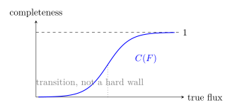
图 9 表示 finite noise 使 flux limit 成为平滑转变;不同背景和 crowding 区域有不同 \(C(F,\mathbf r)\)。
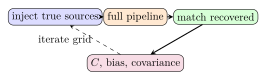
图 10 给出 injection–recovery closure loop;synthetic population 必须覆盖真实的 flux、size、color 与 position 维度。
Worked Examples / 完整例题
Example 1 — 口径、集光与 diffraction resolution
已知: 比较 \(D_1=1.00\,\mathrm m\) 与 \(D_2=4.00\,\mathrm m\) 的理想圆孔,在 \(\lambda=550\,\mathrm{nm}\)。
系统: 相同 throughput、exposure 与 source;忽略遮挡和 seeing。
模型: area ratio 与 Rayleigh criterion。
\[\frac{A_2}{A_1}=\left(\frac{D_2}{D_1}\right)^2=16.\]
\[\theta_2=1.22\frac{550\times10^{-9}}{4.00}\,\mathrm{rad}=1.68\times10^{-7}\,\mathrm{rad}=0.0346''.\]
\(1\) m telescope 的 diffraction scale 为 \(0.138''\),即四倍宽。
检查: 更大 aperture 收 16 倍光、理想角尺度缩小 4 倍;若 ground seeing 为 \(0.8''\) 且无 AO,两台实际图像可能都 seeing-limited。
Example 2 — Background-limited exposure scaling
已知: 一次 \(t_1=300\,\mathrm s\) 曝光中 source \(S_1=900\) counts、background within aperture \(B_1=8100\) counts,其他噪声可忽略。求 SNR;要达 SNR 18 需多长时间?
系统与模型: source/background rates constant,Poisson independent;\(S,B\propto t\)。
\[\mathrm{SNR}_1=\frac{900}{\sqrt{900+8100}}=9.49.\]
在此模型中 \(\mathrm{SNR}\propto\sqrt t\):
\[t_2=t_1\left(\frac{18}{9.49}\right)^2=1.08\times10^3\,\mathrm s.\]
即约 \(18.0\,\mathrm{min}\)。
检查: 若存在 calibration floor,实际时间会更长且最终饱和;不能把此 scaling 外推到无限曝光。
Example 3 — Spectral resolving power 与速度尺度
已知: spectrograph 在 \(\lambda=600.0\,\mathrm{nm}\) 有 \(R=30{,}000\)。求一个 resolution element 的 \(\Delta\lambda\) 和对应低速 Doppler scale。
系统: wavelength calibration 已完成;velocity scale 只表示 instrumental resolution element,不等于 centroid precision。
方程:
\[\Delta\lambda=\frac{\lambda}{R}=0.0200\,\mathrm{nm},\]
\[\Delta v\simeq c\frac{\Delta\lambda}{\lambda}=\frac{c}{R}=9.99\,\mathrm{km\,s^{-1}}.\]
检查: 高 SNR、多条线和稳定 calibration 可把 centroid 测到 resolution element 的一小部分;但这不违反 \(R\),因为“分辨两条线”与“估单线中心”是不同任务。
Example 4 — Interferometer 的细尺度与缺失大尺度
已知: \(\lambda=0.060\,\mathrm m\),projected \(B_{\max}=10.0\,\mathrm{km}\),\(B_{\min}=30.0\,\mathrm m\)。用数量级关系估 angular resolution 和 largest recoverable scale。
系统: narrow-field synthesis array;忽略 weighting factor 和 projection variation。
方程:
\[\theta_{\mathrm{res}}\sim\frac{0.060}{1.00\times10^4}=6.0\times10^{-6}\,\mathrm{rad}=1.24'',\]
\[\theta_{\mathrm{large}}\sim\frac{0.060}{30.0}=2.0\times10^{-3}\,\mathrm{rad}=6.9'.\]
检查: 更长 \(B_{\max}\) 改善细节,但若 \(B_{\min}\) 不变,不会恢复更大平滑结构。实际 coefficients 依 array layout、weighting 和 image-fidelity criterion。
Lesson synthesis / 课程综合
一个可审计的观测流程应明确:
- 由 science question 决定 wavelength、field、resolution、cadence、polarization 与 spectral requirements;
- 用 source + background + detector model 预测 SNR,而不是只比较 aperture;
- 选择 ground/space、single aperture/interferometer,并记录 inaccessible modes;
- 以 standards 和 housekeeping data 估计 \(\mathbf R(\boldsymbol\gamma)\);
- 对 calibrated data 做 inference,并传播 covariance 与 PSF/throughput uncertainty;
- 用 injection–recovery 和 null tests 测 selection、completeness、false positives 与 bias;
- 发布数据时附 units、WCS、filter curve、PSF、mask、selection function 和 provenance。
Formula-and-decision table / 公式与决策表
| Need | Relation | Use when | Main limitation |
|---|---|---|---|
| collecting area | \(A=\pi D^2/4\) | circular unobscured aperture | blockage and throughput |
| diffraction scale | \(\theta\simeq1.22\lambda/D\) | ideal circular pupil | seeing, aberration, algorithm |
| count SNR | \(S/\sqrt{S+B+\cdots}\) | independent calibrated noise terms | correlated/systematic noise |
| spectral resolution | \(R=\lambda/\Delta\lambda\) | one stated definition of \(\Delta\lambda\) | line-spread function sampling |
| synthesis resolution | \(\theta\sim\lambda/B_{\max}\) | projected baseline coverage | weighting and \(uv\) gaps |
| completeness | \(C=P(\mathrm{selected}\mid\mathrm{true})\) | full pipeline and population dimensions | injection realism |
Model boundaries / 模型边界
- Aperture area alone does not determine limiting flux; background surface brightness, PSF, throughput and source extension matter.
- Rayleigh criterion is a convention for two ideal point sources. Model fitting can yield different thresholds but cannot invent absent information.
- Adaptive optics is anisoplanatic and band-limited; space platforms retain thermal, radiation and calibration constraints.
- Spectrograph \(R\) does not uniquely set radial-velocity precision; wavelength stability, line content and SNR are essential.
- Fourier inversion from incomplete \(uv\) coverage is non-unique. Deconvolution uses priors/regularization and can create artifacts.
- A catalog-level cut cannot be corrected by a single scalar completeness if detection depends on multidimensional properties and position. Inverse-completeness weighting is undefined on zero-support regions and unstable where \(C\) is very small; measurement scatter requires a response kernel.
Misconception clinic / 误区诊所
- “放大倍数越高望远镜越好。” 关键物理量是 aperture、PSF、sampling 与 SNR;空放大不增加信息。
- “空间望远镜总比地面望远镜大而灵敏。” 空间消除大气但受 launch/cost;地面可有更大 aperture,两者优势随 band/task 改变。
- “长曝光总能让 SNR 任意增长。” systematic floor、confusion、cosmic rays 和 source variability 会破坏 \(\sqrt t\) scaling。
- “干涉阵列等于一个实心巨镜。” 它匹配某些 angular resolution,却没有填满 aperture 的 collecting area 和 Fourier modes。
- “CLEAN 后图像就是真实天空。” deconvolution 是受采样和先验约束的估计;missing short spacings 仍缺失。
- “超过 5 sigma 的 catalog 就没有选择偏差。” threshold、noise fluctuations、crowding 和 population distribution 仍改变被选样本。
Practice and retrieval / 练习与提取
- [K01 定量] 口径从 2 m 增至 6 m,理想 collecting area 与 fixed-\(\lambda\) diffraction scale 各变多少?
- [K01 建模] 写出 source、sky、dark 与 read noise 均存在时的 SNR,并说明哪些项随曝光时间线性增长。
- [K02 概念] 给出一个必须在空间观测的 band 和一个地面更有工程优势的任务,并说明理由。
- [K02 边界] AO 为什么不能消除 infrared sky thermal background?
- [K03 定量] \(R=5000\) 的 spectrograph 在 \(500\,\mathrm{nm}\) 的 \(\Delta\lambda\) 是多少?
- [K03 概念] Photometry 与 spectroscopy 对 photons 的信息分配有什么 trade-off?
- [K04 定量] \(\lambda=0.21\,\mathrm m\)、\(B_{\max}=36\,\mathrm{km}\),估 resolution,单位 arcsec。
- [K04 判断] 延长 \(B_{\max}\) 但保持 \(B_{\min}\),能否改善 diffuse large-scale recovery?
- [K05 定义] 1000 个注入源中找回 800 个;catalog 900 entries 中估计 720 个真实。求 completeness 与 purity。
- [综合设计] 设计一次 faint extended galaxy survey 的最低校准与 selection validation 清单。
Answer 1
Area ratio \(=(6/2)^2=9\);diffraction scale ratio \(=2/6=1/3\)。在相同 \(\lambda\) 的理想情况下收光 9 倍、PSF angular scale 缩至三分之一。
Answer 2
\[\mathrm{SNR}=\frac{S}{\sqrt{S+B+n_{\mathrm{pix}}(D_{\mathrm{dark}}+N_{\mathrm{read}}\sigma_{\mathrm{read}}^2)}}.\] 固定 rates 下 \(S,B,D_{\mathrm{dark}}\propto t\);read variance 随读出次数而非单次曝光时长线性变化。
Answer 3
例如大部分 X-ray 被大气吸收,需空间平台;大视场可见光时域 survey 可在地面建超大口径、频繁维护且成本较低。答案必须绑定 wavelength 与 science metric。
Answer 4
AO 校正到达 wavefront 的 phase distortion;它不降低大气、望远镜和周围环境自身发出的 thermal photons,也不恢复已被吸收的 photons。
Answer 5
\[\Delta\lambda=\lambda/R=500\,\mathrm{nm}/5000=0.100\,\mathrm{nm}.\]
Answer 6
Photometry 把宽 band photons 汇总,通常获得更高 SNR 与时间效率但 wavelength 信息粗;spectroscopy 分到许多 bins,可见 lines/velocity/composition,但每 bin photons 少、曝光更长。
Answer 7
\[\theta\sim\frac{0.21}{3.6\times10^4}=5.83\times10^{-6}\,\mathrm{rad}=1.20''.\] 实际 synthesized beam 依 weighting 与 projected coverage。
Answer 8
不能。Fine resolution 改善,但 large-scale response 主要由 short baselines 控制;若 \(B_{\min}\) 不变,missing short spacings 仍在。
Answer 9
Completeness \(=800/1000=0.80\);purity \(=720/900=0.80\)。两者数值相同纯属本题数据巧合,分母与问题不同。
Answer 10
至少包括 bias/dark/flat、astrometric/photometric zero points、PSF spatial variation、sky subtraction、surface-brightness dependent injection–recovery、crowding/blending、mask、false detections、color/size dependence、correlated noise、repeat-field/null tests,以及公开 \(C(F,r_e,color,\mathbf r)\)。
Exit ticket / 课末检核
- 某阵列给出漂亮的 high-resolution image,却比 single dish 少很多 integrated flux。用 Fourier sampling 解释,并提出能闭合 flux budget 的观测方案。
- 一份 catalog 宣称“90% complete to magnitude 24”。写出至少五个必须追问的限定词,判断这句话是否可复现。
References and source notes / 参考资料与来源说明
- OpenStax, Astronomy 2e, 6.1 Telescopes — collecting area、optical system 与 telescope functions;accessed 2026-08-30.
- OpenStax, Astronomy 2e, 6.2 Telescopes Today — ground sites、seeing、adaptive optics 与 space observing;accessed 2026-08-30.
- OpenStax, Astronomy 2e, 6.3 Visible-Light Detectors and Instruments — detectors、long exposure 与 spectroscopy trade-off;accessed 2026-08-30.
- OpenStax, Astronomy 2e, 6.4 Radio Telescopes — interferometry、baseline 与 synthesis arrays;accessed 2026-08-30.
- NASA Webb, Telescope Overview — primary mirror、collecting area 与 space telescope design;accessed 2026-08-30.
- NRAO, An Overview of the VLA — visibility、correlation、array configurations;accessed 2026-08-30.
- NRAO, Limitations on Imaging Performance — image fidelity、missing large-scale structure 与 wide-field limitations;accessed 2026-08-30.
- NASA/IPAC IRSA, 2MASS All-Sky Data Release User's Guide: Sensitivity and Completeness — repeated-calibration completeness、crowding 与 flux limits;accessed 2026-08-30.
- S. Everett et al. (DES Collaboration), “Dark Energy Survey Year 3 Results: Measuring the Survey Transfer Function with Balrog,” ApJS 258, 15 (2022), publisher DOI and open preprint — image-level injection、production-like detection/measurement、truth matching、completeness 与 measurement-bias recovery;accessed 2026-08-30.
所有 TikZ 均为依据 measurement equations 原创的教学图;未复制 telescope photographs 或官方 figures。设施数值只用于来源语境,正文例题采用自洽的教学参数。
Source-to-content map / 来源—内容映射
| Source | Used for | Knowledge ID / Section | Model boundary or convention |
|---|---|---|---|
| OpenStax 6.1 | area, focusing, detector chain | K01 | ideal aperture vs real throughput |
| OpenStax 6.2 | seeing, AO, ground/space | K02 | wavelength- and site-dependent |
| OpenStax 6.3 | detectors and spectroscopy | K01, K03 | photon bins and thermal background |
| OpenStax 6.4 | interferometry | K04 | baseline is not filled aperture |
| NASA Webb overview | space mirror and area | K01, K02 | engineering context, not universal ranking |
| NRAO VLA overview/limitations | visibilities, \(uv\) sampling, missing modes | K04 | projected baselines and image fidelity |
| 2MASS User's Guide | repeated-observation completeness and reliability | K05 | position, crowding and magnitude dependence; not an image-injection source |
| Everett et al. Balrog | image-level injection, full pipeline, truth matching, completeness and bias | K05, Figure 10 | closure is conditional on injected-population and pipeline fidelity |
复习与拓展
- 与前课连接:flux、color、line shift 都是经过 response operator 后的估计量;下一步 astrophysical modeling 必须继承 calibration covariance。
- 与 Unit 12.2 连接:planet formation 与 orbital architecture 的观测样本受 transit geometry、radial-velocity threshold 和 imaging contrast selection 影响。
- 后续可扩展:Fisher information、optimal extraction、PSF photometry、CASA imaging、Bayesian deconvolution、survey window functions 与 reproducible data provenance。