
Learning objectives / 学习目标
学完本课后,你应能:
- 解释 long-range Coulomb force 为什么产生以许多小角散射累积而成的 collision time,并说明 Coulomb logarithm 的上下 cutoff;
- 使用明确 convention 的 collision frequency,检查其 \(nT^{-3/2}\) scaling、mean free path 与弱耦合边界;
- 从含 drag 的 species momentum balance 推导 mobility、conductivity、Fick diffusion 和 Einstein relation;
- 从零净电流条件推导 singly ionized plasma 的 ambipolar field 与 \(D_a\),辨别它何时失效;
- 用 magnetization parameter \(\beta_s=\omega_{cs}/\nu_s\) 判断 parallel、Pedersen、Hall 与 classical cross-field transport,并区分 classical 与 turbulent transport。
Prerequisites / 先修知识
- Single-Particle Motion:gyrofrequency、gyroradius 与 guiding center;
- Plasma State and Characteristic Scales:Debye length、plasma parameter 与 quasineutrality;
- random walk、Fick's law、gradient 与 elementary probability;
- Lorentz force、current density、thermal speed 和 SI dimensional analysis。
Scope and conventions / 范围与约定
- 默认 nonrelativistic、weakly coupled、fully ionized 或弱电离且可指定中性 drag 的 plasma;温度 \(T_s\) 在公式中用 kelvin 时写 \(k_BT_s\),用 eV 时明确换算。
- 本课的 \(\nu_s\) 是用于 momentum/deflection estimate 的 effective frequency;不同资料对 \(90^\circ\) deflection、slowing-down、energy-equilibration frequency 的数值系数不同,不能只比较符号名称。
- 只在 local, near-Maxwellian, linear-response regime 使用 scalar \(D,\mu,\sigma\);磁化后它们一般是 tensor。
- \(\mathbf B=B\hat z\);若有一维 density gradient,取 \(+x\) 为密度增加方向,diffusive flux 指 \(-x\)。
- classical transport 来自 binary Coulomb/neutral collisions;drift-wave turbulence、neoclassical toroidal effects 与 nonlocal transport 只标出接口,不混入 classical coefficient。
Notation and modeling contract / 符号与建模契约
| Symbol | Meaning | SI / convention |
|---|---|---|
| \(n_s,q_s,m_s\) | species density, charge, mass | \(\mathrm{m^{-3}}\), C, kg |
| \(\nu_s,\tau_s\) | effective collision frequency and time | \(\mathrm{s^{-1}}\), s |
| \(\ln\Lambda\) | Coulomb logarithm | dimensionless |
| \(\ell_s=v_{ts}/\nu_s\) | mean free path estimate | m |
| \(\mu_s\) | positive mobility magnitude | \(\mathrm{m^2\,V^{-1}\,s^{-1}}\) |
| \(D_s\) | particle diffusivity | \(\mathrm{m^2\,s^{-1}}\) |
| \(\sigma\) | electrical conductivity | \(\mathrm{S\,m^{-1}}\) |
| \(\boldsymbol\Gamma_s=n_s\mathbf u_s\) | particle flux density | \(\mathrm{m^{-2}\,s^{-1}}\) |
| \(\beta_s=\omega_{cs}/\nu_s\) | Hall or magnetization parameter | dimensionless |
1. Coulomb collisions and collision frequency / 库仑碰撞与碰撞频率
Knowledge ID: P13-U02-L01-K01
1.1 从 binary encounter 到 cumulative deflection
带电粒子的 Rutherford scattering 没有一个天然的短程截面:impact parameter \(b\) 很大的 encounter 单次偏转很小,却数量极多。对许多 statistically independent 小角 kick,transverse velocity change 做 random walk,故 mean-square deflection 随时间线性增加;“collision time”通常定义为累计到 order-one 或 \(90^\circ\) deflection 的时间。
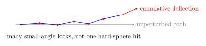
图 1 把 collision 描画为方向扩散;红点表示 encounter 时刻,不表示实际 point contact。
1.2 Coulomb logarithm 与 scaling
弱耦合 plasma 的 transport integral 近似含
\[\ln\Lambda=\ln\left(\frac{b_{\max}}{b_{\min}}\right).\]
\(b_{\max}\) 通常由 Debye shielding 或 finite system/correlation scale 截断;\(b_{\min}\) 取 classical distance of closest approach 与 quantum de Broglie scale 中较大者。若 \(\ln\Lambda\) 不大,独立 binary small-angle picture 本身需重新检验。
对 Maxwellian electron–ion scattering,一种常用 SI deflection-frequency convention 为
\[\nu_{ei}=\frac{4\sqrt{2\pi}}{3} \frac{n_i Z^2 e^4\ln\Lambda} {(4\pi\epsilon_0)^2\sqrt{m_e}(k_BT_e)^{3/2}}.\]
最稳健的物理 scaling 是
\[\nu_{ei}\propto n_i Z^2\ln\Lambda\,T_e^{-3/2}.\]
密度越高 encounter 越频繁;温度越高粒子越快、单次偏转越弱,故 \(T^{-3/2}\) 急剧下降。
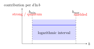
图 2 解释两个 cutoff:每个 logarithmic impact-parameter band 都贡献同一数量级,积分才形成 \(\ln\Lambda\)。
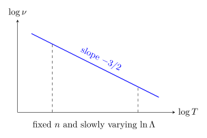
图 3 是 log–log scaling audit;曲线不是某个特定装置的拟合。
2. Conductivity, diffusion, and mobility / 电导、扩散与迁移率
Knowledge ID: P13-U02-L01-K02
2.1 Drag balance 与 mobility/conductivity
在 uniform, unmagnetized, steady, weak-field limit,用 electron drift \(\mathbf u_e\) 相对 ions 的 momentum balance:
\[0=-en_e\mathbf E-m_en_e\nu_{ei}\mathbf u_e.\]
故 electron drift 与 conventional current 分别为
\[\mathbf u_e=-\mu_e\mathbf E, \qquad \mu_e=\frac{e}{m_e\nu_{ei}},\]
\[\mathbf J=-en_e\mathbf u_e=\sigma\mathbf E, \qquad \sigma=\frac{n_e e^2}{m_e\nu_{ei}}.\]
这是 Drude-like estimate;精确 Spitzer–Härm conductivity 要解 linearized kinetic equation,并因 electron–electron collisions 与 distribution distortion 修正 coefficient。
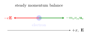
图 4 中 electron drift 逆 \(\mathbf E\),但 conventional current 顺 \(\mathbf E\)。
2.2 Diffusion 与 Einstein relation
一维 isothermal species 的 drift–diffusion flux 可写
\[\Gamma_s=-D_s\frac{dn_s}{dx}+s_s\mu_s n_s E,\]
其中 \(s_s=\operatorname{sgn}(q_s)\),\(\mu_s>0\) 是 mobility magnitude。local Maxwellian 与同一 drag model 给出 Einstein relation:
\[D_s=\mu_s\frac{k_BT_s}{\lvert q_s\rvert} =\frac{k_BT_s}{m_s\nu_s}.\]
它不是任意 nonequilibrium distribution 的恒等式;若 energetic tail、nonlocal mean-free-path 或 anomalous scattering 主导,必须回到 kinetic equation。
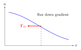
图 5 将 density gradient 与 particle flux 分开;flux 箭头不是单一粒子的轨迹。
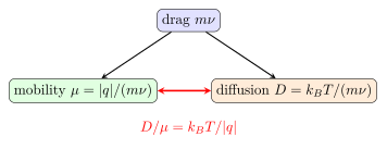
图 6 是 modeling contract:mobility 与 diffusion 必须来自同一 collision model 才能直接用 Einstein relation。
3. Ambipolar diffusion / 双极扩散
Knowledge ID: P13-U02-L01-K03
electron thermal speed 与 free diffusivity 通常远大于 ion 值。若 electrons 先向边界流失,微小 charge separation 会产生 ambipolar electric field,减慢 electrons、加速 ions。超过 Debye scale 后 plasma 近似 quasineutral,open-circuit bulk 中还要求 zero net current:
\[\Gamma_i=\Gamma_e\equiv\Gamma_a.\]
对 singly ionized、isothermal、unmagnetized plasma,令 \(dn/dx\) 为共同 gradient:
\[\Gamma_i=-D_i\frac{dn}{dx}+\mu_i nE,\]
\[\Gamma_e=-D_e\frac{dn}{dx}-\mu_e nE.\]
令两者相等,得到
\[E_a=\frac{D_i-D_e}{(\mu_i+\mu_e)n}\frac{dn}{dx},\]
\[\boxed{D_a=\frac{\mu_eD_i+\mu_iD_e}{\mu_e+\mu_i}}.\]
若 \(\mu_e\gg\mu_i\) 且各自满足 Einstein relation:
\[D_a\simeq D_i\left(1+\frac{T_e}{T_i}\right).\]
这并不意味着 quasineutrality 处处精确;sheath、double layer、very short times、electron attachment 或多离子组分会改变边界与 coefficient。
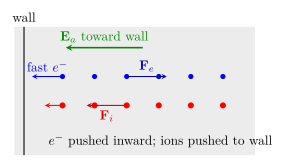
图 7 的 blue/red dots 是 species density markers。wall 在左、plasma interior 在右;\(\mathbf E_a\) 指向 wall,因此 electron electric force 指向 interior、抑制 electron loss,而 positive-ion force 指向 wall、加速 ion loss,二者趋向 coupled flux。
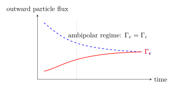
图 8 表示 charge-relaxation transient 后的 equal flux;纵轴不是 current,因为 conventional currents 的 signs 不同。
4. Cross-field transport / 跨磁场输运
Knowledge ID: P13-U02-L01-K04
在 \(\mathbf B=B\hat z\) 中,collision 会随机化 gyrophase 并使 guiding center 每次改变约一个 gyroradius。量级估计为
\[D_{\perp s}\sim \rho_s^2\nu_s \qquad (\omega_{cs}\gg\nu_s).\]
简单 Lorentz-drag model 给出
\[D_{\parallel s}=D_{0s}, \qquad D_{\perp s}=\frac{D_{0s}}{1+\beta_s^2}, \qquad \beta_s=\frac{\omega_{cs}}{\nu_s}.\]
同一 inversion 也产生 Hall response,方向垂直于 applied force 与 \(\mathbf B\)。注意:\(\mathbf E\times\mathbf B\) drift 是 coherent bulk advection,不应直接叫 diffusion;diffusion 是 ensemble spreading,需 gradient 或 stochastic decorrelation。
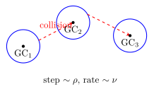
图 9 是 gyrocenter random walk;三个圆是相邻 orbit 段,不是三个粒子。
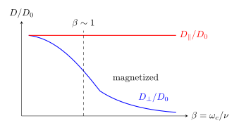
图 10 展示 anisotropy transition;横轴为 schematic logarithmic progression,未声称线性比例。
Worked examples / 完整例题
Worked Example 1 — Electron collision time 与 mean free path
已知: fully ionized hydrogen,\(n_e=n_i=1.00\times10^{18}\ \mathrm{m^{-3}}\),\(T_e=20.0\ \mathrm{eV}\),\(\ln\Lambda=12.0\)。
研究对象: Maxwellian electrons;ions 为 momentum-scattering background。
参考系与方向: plasma rest frame;本题只求 magnitudes。
模型: NRL Formulary 的 practical electron collision-rate convention,输入 \(n_e\) 用 \(\mathrm{cm^{-3}}\)、\(T_e\) 用 eV。
先换算 \(n_e=1.00\times10^{12}\ \mathrm{cm^{-3}}\):
\[\nu_e=2.91\times10^{-6}n_e\ln\Lambda\,T_e^{-3/2} =3.90\times10^5\ \mathrm{s^{-1}}.\]
\[\tau_e=\nu_e^{-1}=2.56\ \mu\mathrm s.\]
取 \(v_{te}=\sqrt{2eT_e/m_e}=2.65\times10^6\ \mathrm{m\,s^{-1}}\):
\[\ell_e=\frac{v_{te}}{\nu_e}=6.79\ \mathrm m.\]
检查: 若温度加倍,忽略 \(\ln\Lambda\) 变化,\(\nu\) 乘 \(2^{-3/2}=0.354\);结果符合 hotter plasma 更 collisionless。三位有效数字。\(\ell_e\) 若接近装置尺度,local transport closure 需谨慎。
Worked Example 2 — Drag-model conductivity
已知: 沿用 Example 1 的 \(n_e\) 与 \(\nu_e\),施加弱 steady electric field。
系统边界: homogeneous bulk,忽略 magnetic field、pressure gradient 与 electron inertia。
模型理由: linear momentum-drag estimate。
\[\sigma=\frac{n_e e^2}{m_e\nu_e} =\frac{(1.00\times10^{18})(1.602\times10^{-19})^2} {(9.109\times10^{-31})(3.90\times10^5)} =72.1\ \mathrm{S\,m^{-1}}.\]
若 \(E=2.00\ \mathrm{V\,m^{-1}}\),则 \(J=\sigma E=144\ \mathrm{A\,m^{-2}}\),方向沿 \(\mathbf E\)。
检查: \(ne^2/(m\nu)\) 为 \(\mathrm{A\,V^{-1}\,m^{-1}}\);electron drift 逆场但 current 顺场。此数值是简单 drag coefficient,不冒充完整 Spitzer–Härm result。
Worked Example 3 — Ambipolar diffusion coefficient
已知: weakly ionized singly charged plasma,\(T_e=3.00\ \mathrm{eV}\),\(T_i=0.0300\ \mathrm{eV}\),free ion diffusivity \(D_i=2.00\times10^{-2}\ \mathrm{m^2\,s^{-1}}\),且 \(\mu_e\gg\mu_i\)。
系统: quasineutral bulk between sheaths,open circuit;一维 density gradient。
模型: isothermal Einstein relations,single positive ion species。
\[D_a\simeq D_i\left(1+\frac{T_e}{T_i}\right) =(2.00\times10^{-2})(1+100) =2.02\ \mathrm{m^2\,s^{-1}}.\]
若 gradient scale \(L_n=0.500\ \mathrm m\),diffusion time estimate:
\[\tau_D\sim\frac{L_n^2}{D_a}=0.124\ \mathrm s.\]
检查: \(D_a>D_i\),因为 field 加速 ions;但它远小于 arbitrary free-electron coefficient。若 boundary supplies net current,\(\Gamma_i=\Gamma_e\) 条件不再自动成立。
Worked Example 4 — Magnetized cross-field suppression
已知: electron \(D_0=10.0\ \mathrm{m^2\,s^{-1}}\),\(\nu_e=1.00\times10^6\ \mathrm{s^{-1}}\),\(B=0.0200\ \mathrm T\)。
坐标: \(\mathbf B=B\hat z\);比较 \(z\) 与 \(x\) diffusion。
模型: Lorentz-drag transport tensor,\(\omega_{ce}=eB/m_e\)。
\[\omega_{ce}=3.52\times10^9\ \mathrm{s^{-1}}, \qquad \beta_e=3.52\times10^3.\]
\[D_{\perp e}=\frac{D_0}{1+\beta_e^2} =8.07\times10^{-7}\ \mathrm{m^2\,s^{-1}}, \qquad D_{\parallel e}=10.0\ \mathrm{m^2\,s^{-1}}.\]
检查: strong-field limit gives \(D_0/\beta^2\),与 \(\rho_e^2\nu_e\) scaling 一致。anisotropy ratio \(D_\parallel/D_\perp=1.24\times10^7\);真实装置若测得更大 cross-field loss,可能有 turbulence、geometry 或 wall effects,不能通过篡改 \(\nu\) 解释。
Lesson synthesis / 全课整合
输运建模流程:先定义 collision frequency convention → 核对 \(\ln\Lambda\) 与 weak-coupling → 比较 \(\ell/L\) 判断 local closure → 写 species vector momentum balance → 在无磁场求 mobility/conductivity/diffusion → 用 current/boundary condition 决定 ambipolar field → 有磁场时计算 \(\omega_c/\nu\) 并使用 tensor → 将 classical prediction 与 measured transport 分开比较。
Formula-and-decision table / 公式与决策表
| Need | Relation | Use only when | Main caution |
|---|---|---|---|
| collision scaling | \(\nu_{ei}\propto n_iZ^2\ln\Lambda T_e^{-3/2}\) | weakly coupled Maxwellian plasma | coefficients depend on collision-time definition |
| mean free path | \(\ell=v_t/\nu\) | specified thermal-speed convention | local closure also needs \(\ell/L\ll1\) |
| conductivity estimate | \(\sigma=n_e e^2/(m_e\nu_{ei})\) | weak field, linear drag | Spitzer coefficient requires kinetic solution |
| Einstein relation | \(D_s=\mu_s k_BT_s/\lvert q_s\rvert\) | local equilibrium and common drag model | not universal in nonequilibrium plasma |
| ambipolar diffusion | \(D_a=(\mu_eD_i+\mu_iD_e)/(\mu_e+\mu_i)\) | singly ionized, quasineutral, zero current | sheaths and multiple ions alter it |
| magnetization | \(\beta_s=\omega_{cs}/\nu_s\) | local uniform \(B\) estimate | species have different \(\beta_s\) |
| cross-field diffusion | \(D_\perp=D_0/(1+\beta^2)\) | simple collisional tensor | does not include turbulent transport |
Model boundaries / 模型边界
- Strong coupling, degeneracy, relativistic temperatures or \(\ln\Lambda\sim1\) require models beyond weak-coupling Coulomb kinetics.
- A single \(\nu\) cannot simultaneously represent pitch-angle scattering, slowing down and energy exchange with exact coefficients.
- If \(\ell/L\gtrsim1\),Fourier/Fick local laws become nonlocal; boundary distribution matters.
- Ambipolar theory applies to quasineutral bulk, not to sheath-scale charge separation;external circuits may impose nonzero current。
- Strongly magnetized toroidal plasmas have neoclassical orbit effects beyond uniform-field \(D_\perp\)。
- Turbulent cross-field flux can dominate classical random walk;this is revisited in Lesson 13.3.2。
Misconception clinic / 易错概念诊所
| Misconception | Correction |
|---|---|
| collision means one close impact | Coulomb relaxation usually accumulates many small-angle encounters |
| hotter plasma collides more because particles move faster | deflection weakens faster; \(\nu\propto T^{-3/2}\) |
| conductivity is independent of collision model | \(\sigma\) depends on momentum relaxation and kinetic distortion |
| ambipolar means electric field is zero | a small self-consistent field is precisely what locks electron and ion fluxes |
| quasineutral means \(n_i=n_e\) at every point | finite Debye-scale charge imbalance supports \(E_a\) and sheaths |
| \(\mathbf E\times\mathbf B\) drift is diffusion | coherent drift translates a distribution; diffusion measures spreading down gradients |
| magnetic field eliminates all perpendicular loss | it suppresses classical transport but collisions, geometry and turbulence remain |
Practice and retrieval / 练习与检索
- [K01] 固定 \(n\) 与 \(\ln\Lambda\),\(T_e\) 增为原来的 4 倍时 \(\nu_{ei}\) 如何变化?
Answer 1
\(\nu\propto T^{-3/2}\),所以变为 \(4^{-3/2}=1/8\)。
- [K01] 为什么 \(b_{\max}\) 不能取 infinity?
Answer 2
Debye shielding 或有限 correlation/system scale 会屏蔽远距 encounter;否则 logarithmic integral 无物理上限。
- [K01] \(\nu=2.0\times10^5\ \mathrm{s^{-1}}\)、\(v_t=1.0\times10^6\ \mathrm{m\,s^{-1}}\),求 \(\tau\) 与 \(\ell\)。
Answer 3
\(\tau=1/\nu=5.0\ \mu\mathrm s\),\(\ell=v_t/\nu=5.0\ \mathrm m\)。
- [K02] electron drift 为什么与 conventional current 方向相反?
Answer 4
electron charge 为负,\(\mathbf J_e=q_en_e\mathbf u_e\);两个负号使 current 沿 \(\mathbf E\)。
- [K02] 若 \(\nu\) 加倍而其他量不变,\(\mu,D,\sigma\) 如何变?
Answer 5
在本课 drag model 中三者均与 \(1/\nu\) 成正比,所以都减半。
- [K03] ambipolar field 对 fast electrons 和 slow positive ions 分别做什么?
Answer 6
它把 electrons 拉回 plasma、把 ions 向外推,使两者 particle flux 相等而 bulk 保持 quasineutral。
- [K03] \(T_e=T_i\) 且 \(\mu_e\gg\mu_i\) 时,近似 \(D_a/D_i\) 是多少?
Answer 7
\(D_a\simeq D_i(1+T_e/T_i)=2D_i\)。
- [K04] \(\omega_c/\nu=10\) 时 \(D_\perp/D_0\)?
Answer 8
\(D_\perp/D_0=1/(1+10^2)=1/101=9.90\times10^{-3}\)。
- [K04] strong magnetization 下若 collision frequency 加倍且 \(v_t,B\) 不变,\(D_\perp\sim\rho^2\nu\) 如何变化?
Answer 9
\(\rho=v_t/\omega_c\) 不变,所以 \(D_\perp\) 加倍;collision 既造成阻力,也提供跨 gyrocenter 的随机 step。
- [综合] 某实验的 measured \(D_\perp\) 比 classical estimate 大 \(10^4\) 倍。能否直接把差异称为 Coulomb collision coefficient error?
Answer 10
不能。应先审计 geometry、neutral collisions、boundaries 与 diagnostics,再考虑 drift-wave turbulence 或其他 anomalous transport;Coulomb logarithm 的缓慢变化不可能自然提供 \(10^4\) factor。
Exit ticket / 迁移检验
对一个给出 \(n,T,B,L\) 的 plasma,写出决定“collisionless / local collisional / magnetized transport / ambipolar”描述的四步判据。
Exit-ticket benchmark
先算并声明 \(\nu\) convention 与 \(\ell=v_t/\nu\);比较 \(\ell/L\);再算 \(\omega_c/\nu\);最后检查 quasineutral bulk、boundary current 与 species flux constraint,决定是否需要 ambipolar field。
References and source notes / 参考资料与使用说明
以下权威直接来源均在 2026-08-31 实际打开核对;正文重新组织,所有 TikZ 依据方程原创绘制,未复制来源插图。
- MIT OpenCourseWare 22.611J, Chapter 3 — Collisions in Plasmas — small-angle Coulomb scattering、collision times 与 cross-field random walk。
- MIT OpenCourseWare 16.55, Lecture 15 — Maxwellian Collisions — conductivity tensor、mobility 与 ambipolar diffusion。
- MIT OpenCourseWare 22.616, Collisions and Transport Theory II — Spitzer–Härm conductivity 作为 kinetic transport problem。
- Richard Fitzpatrick, UT Austin, Coulomb Logarithm — impact-parameter cutoffs 与 weak-coupling interpretation。
- Richard Fitzpatrick, UT Austin, Magnetized Limit — parallel/perpendicular collisional transport anisotropy。
- U.S. Naval Research Laboratory, 2023 NRL Plasma Formulary — practical collision-rate coefficients and unit conventions。
- Princeton Plasma Physics Laboratory, Principles of Transport in Multicomponent Plasmas — ambipolar polarization、limits with additional species。
Source-to-content map
| Source | Used for | Knowledge ID / Section | Model boundary or convention |
|---|---|---|---|
| MIT 22.611J Ch. 3 | small-angle collision and gyrocenter random walk | K01, K04 | weakly coupled, classical binary transport |
| MIT 16.55 L15 | mobility tensor and ambipolar derivation | K02–K04 | Maxwellian, linear momentum balance |
| MIT 22.616 Part II | conductivity as kinetic response | K02 | Spitzer–Härm coefficient beyond simple drag |
| Fitzpatrick Coulomb Log | \(b_{\min},b_{\max},\ln\Lambda\) | K01 | logarithmic many-body screening correction |
| Fitzpatrick Magnetized Limit | anisotropic coefficients | K04 | collisional magnetized closure |
| NRL 2023 | numerical coefficient and constants | Worked 1–2 | density in \(\mathrm{cm^{-3}}\), temperature in eV |
| PPPL multicomponent transport | ambipolar field and failure modes | K03 | quasineutral, species-dependent assumptions |
复习与拓展
- Lesson 13.2.2 将把 scalar collision frequency 替换为 phase-space collision operator,并解释 distribution distortion 与 Landau resonance。
- Lesson 13.2.3 将由 species momentum equations 组合出 generalized Ohm law、resistive diffusion 与 MHD ordering。
- Lesson 13.3.2 将比较 classical \(D_\perp\) 与 fluctuation correlation \(\langle\tilde n\tilde v_r\rangle\) 产生的 turbulent flux。