
Learning objectives / 学习目标
学完本课后,你应能:
- 从节点—边数据建立 adjacency matrix,计算 degree、shortest-path length、connected component 与 clustering coefficient;
- 区分 Erdős–Rényi random、Watts–Strogatz small-world 与 preferential-attachment scale-free model,并说明模型不等于真实网络;
- 从守恒通量推导 graph diffusion equation,使用 Laplacian spectrum 判断 mixing timescale;
- 用 branching/percolation criterion 判断传播阈值,区分 simple contagion、threshold cascade 与 flow overload;
- 定义 robustness observable,比较 random failure 与 targeted removal,并说明控制结论依赖具体动力学;
- 计算 Shannon entropy、conditional entropy 与 mutual information,避免把 entropy 无条件等同于“混乱”。
Prerequisites / 先修知识
- Emergence and Collective Dynamics 中的 local rule、collective state、criticality 与 model hierarchy;
- probability mass function、expectation、binomial/Poisson distribution;
- matrix multiplication、eigenvalue/eigenvector、ordinary differential equations;
- diffusion、conservation law、phase transition 与 logarithm。
Scope and conventions / 范围与约定
- 除非特别声明,图 \(G=(V,E)\) 是 finite、simple、undirected、unweighted graph;\(N=\lvert V\rvert\)、\(M=\lvert E\rvert\)。
- adjacency matrix 记为 \(A\),degree matrix 记为 \(D\),combinatorial Laplacian 为 \(L=D-A\)。
- path length 只在 connected vertex pairs 间定义;disconnected graph 的“平均距离”必须声明处理方式,不能把 \(\infty\) 偷换成零。
- random graph、small-world、scale-free 是模型家族或统计特征,不是互斥的自然种类;finite data 的 power-law claim 必须检验 cutoff、alternative distributions 与 sampling bias。
- contagion probabilities 属于给定时间窗和边的 transmission model;control 的 actuator、state equation 与 objective 必须先给出。
- information logarithm 使用 base 2,单位为 bit;若使用 natural logarithm,单位为 nat。
Notation and modeling contract / 符号与建模契约
| Symbol | Meaning | Unit / convention |
|---|---|---|
| \(N,M\) | numbers of vertices and edges | 1 |
| \(A_{ij}\) | adjacency entry | 0 or 1 here |
| \(k_i\) | degree of vertex \(i\) | 1 |
| \(d(i,j)\) | shortest-path length | edges |
| \(C_i\) | local clustering coefficient | 1 |
| \(p\) | edge probability in \(G(N,p)\) | 1 |
| \(P(k)\) | degree distribution | 1 |
| \(L=D-A\) | graph Laplacian | 1 |
| \(\lambda_2\) | algebraic connectivity of \(L\) | 1 |
| \(\mathcal T\) | edge transmissibility | 1 |
| \(S(q)\) | giant-component fraction after removal fraction \(q\) | 1 |
| \(H(X)\) | Shannon entropy | bit |
| \(I(X;Y)\) | mutual information | bit |
1. Graph structure, degree, paths, and clustering / 图结构、度、路径与聚类
Knowledge ID: P14-U05-L02-K01
graph 把研究对象抽象为 vertices 与 interactions 抽象为 edges。对 simple undirected graph,
\[A_{ij}= \begin{cases} 1,& \{i,j\}\in E,\\ 0,& \text{otherwise}, \end{cases} \qquad k_i=\sum_j A_{ij}, \qquad \sum_i k_i=2M.\]
最后一个等式是 handshake lemma:每条无向边在 degree sum 中被两端各数一次。它也是数据质检规则;若 degree sum 为奇数,edge list 或计数必有错误。
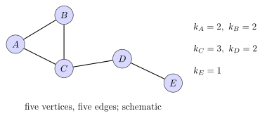
图 1 让 degree 成为“局部连接数”而不是空间邻近程度;页面上的几何距离不属于 graph,除非另行赋予 edge length。
从 \(i\) 到 \(j\) 的 path 是相邻 vertices 的序列;shortest-path length \(d(i,j)\) 是最少边数。connected graph 的 characteristic path length 可写
\[\ell=\frac{2}{N(N-1)}\sum_{i<j}d(i,j).\]
local clustering 衡量 vertex 的 neighbors 彼此是否相连。若 \(k_i\ge2\),令 \(t_i\) 为 neighbors 之间实际边数,则
\[C_i=\frac{2t_i}{k_i(k_i-1)}.\]
本课约定 \(k_i<2\) 时 \(C_i=0\);有些软件选择 undefined,因此跨资料比较前必须核对 convention。network-average \(\bar C=N^{-1}\sum_iC_i\) 与 global transitivity \(3\times(\text{triangles})/(\text{connected triples})\) 不同。
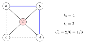
图 2 中 blue edges 是 neighbor pairs 中已闭合的两对,gray dashed lines 只表示可能边而非真实边。
2. Random, small-world, and scale-free networks / 随机、小世界与无标度网络
Knowledge ID: P14-U05-L02-K02
在 Erdős–Rényi \(G(N,p)\) model 中,每一对 vertices 独立地以 probability \(p\) 连边:
\[\Pr(k)=\binom{N-1}{k}p^k(1-p)^{N-1-k}, \qquad \langle k\rangle=p(N-1).\]
当 \(N\) 大、\(p\) 小而 \(\langle k\rangle\) 固定时,degree distribution 近 Poisson。该模型是有用 null model,却缺少许多真实网络的 clustering、degree correlation、spatial cost 与 growth history。
Watts–Strogatz model 从 regular ring lattice 出发,以 rewiring probability \(r\) 引入 shortcuts。在中间 regime,\(\ell\) 可大幅下降而 clustering 仍高,这才是 small-world 的核心组合:short paths plus substantial clustering,不是仅仅“网络不大”。
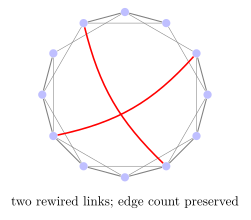
图 3 删除原 ring edges \(v_1v_2\)、\(v_4v_5\),再用两条 red long-range links 取代,因此 edge count 与 mean degree 不变;少量 rewiring 仍可显著缩短远端 pairs 的 geodesic distance。
scale-free 通常指某一范围内
\[P(k)\propto k^{-\gamma}.\]
Barabási–Albert model 用 growth 与 preferential attachment 产生 heavy tail:
\[\Pi_i=\frac{k_i}{\sum_jk_j}.\]
但“直线 log–log 图”不足以证明 power law;应使用 maximum-likelihood fitting、goodness-of-fit 与 alternative-distribution comparison,并检查 finite-size cutoff、measurement threshold 与 sampling bias。lognormal 或 stretched exponential 也可能产生近似直线。真实网络还常 directed、weighted、temporal and multilayer。
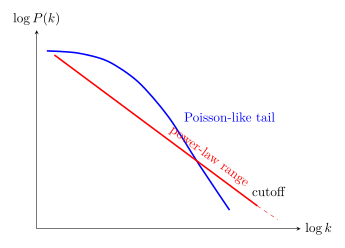
图 4 对比 log–log axes 上的 thin-tailed 与 power-law-like behavior;red dashed cutoff 强调 finite network 没有无限 degree。
3. Diffusion, contagion, and percolation on networks / 网络上的扩散、传播与渗流
Knowledge ID: P14-U05-L02-K03
令 \(x_i\) 是 vertex \(i\) 上的 conserved scalar。每条 edge 的 diffusive flux 与 difference \(x_i-x_j\) 成正比,则
\[\frac{dx_i}{dt} =-\kappa\sum_jA_{ij}(x_i-x_j), \qquad \dot{\mathbf x}=-\kappa L\mathbf x.\]
对 undirected graph,\(\mathbf 1^{\mathsf T}L=0\),所以 \(\sum_ix_i\) conserved。若 graph connected,\(\lambda_1=0<\lambda_2\);slowest nonuniform mode roughly decays as \(e^{-\kappa\lambda_2t}\)。\(\lambda_2\) 大通常意味着 faster linear mixing,但 nonlinear contagion 不由一个 eigenvalue 完全决定。
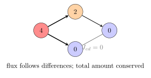
图 5 是一个 instant 的 flux-direction map;arrows 不是 permanent directed edges,concentration order 改变后 flux 可反向。由于图中 \(x_c=x_d=0\),edge \(c-d\) 只画成 gray undirected connection,并显式标记 instantaneous flux \(J_{cd}=0\)。
simple contagion 把每条 active contact 的 transmission 视为 probability event;complex/threshold contagion 则需多个 neighbors 或 cumulative dose。SIR process 在 locally tree-like network 上可与 bond percolation 对应:每条 edge 以 transmissibility \(\mathcal T\) 被“占据”。configuration-model threshold 为
\[\mathcal T_c =\frac{\langle k\rangle} {\langle k^2\rangle-\langle k\rangle}.\]
只有满足 locally tree-like、uncorrelated degree、specified infectious process 等条件才可直接使用。lattice、clustering、degree correlations、time-varying contacts 与 repeated exposure 会改变 threshold。
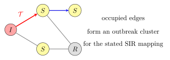
图 6 把 infection history 映射为 occupied-edge cluster;它不是说 infection 真正沿静态边瞬时完成。
4. Robustness, cascades, and control / 鲁棒性、级联与控制
Knowledge ID: P14-U05-L02-K04
“robust” 必须对应 observable 与 perturbation ensemble。例如,删除 fraction \(q\) vertices 后 giant connected component fraction
\[S(q)=\frac{N_{\mathrm{giant}}(q)}{N_{\mathrm{initial}}}\]
测 connectivity robustness,却不等于 flow capacity、latency、synchrony 或 safety。heterogeneous hub network 可能对 uniform random failures 相对稳健,却对 targeted high-degree removal 脆弱;这是一类模型结果,不是所有 scale-free network 的无条件定律。
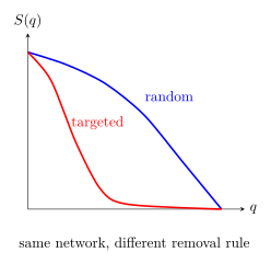
图 7 是 qualitative robustness curves,不宣称 universal numerical values。
cascade 需要 state-dependent coupling。若 edge \(e\) 有 load \(F_e\) 与 capacity \(C_e\),初始 failure 可使 flow reroute;当 \(F_e>C_e\) 时二次 failure 发生并继续传播。仅增加 connectivity 可能既提供 redundancy,也可能增加 long-range propagation channel。
control 要写出 dynamics:
\[\dot{\mathbf x}=f(\mathbf x,A)+B\mathbf u,\]
并声明 controllability、energy、time horizon、constraints 与 measurement。线性 structural controllability 的 driver-node count 不能直接替代 nonlinear system 的实际可控性。
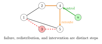
图 8 中 red dashed branch 表示失效路径,orange arrow 沿仍存在的 \(2-4-5\) edges 表示 load redistribution,green input 表示明确 actuator;三者不能混成一条“cascade arrow”。
5. Entropy and information measures / 熵与信息度量
Knowledge ID: P14-U05-L02-K05
离散 random variable \(X\) 的 Shannon entropy 是
\[H(X)=-\sum_xp(x)\log_2p(x),\]
约定 \(0\log_20=0\)。entropy 是对给定 probability model 的平均 code-length lower bound/information uncertainty;它不单独说明 thermodynamic entropy、semantic value 或 causal influence。
joint 与 conditional entropy 满足
\[H(X,Y)=H(X)+H(Y\mid X),\]
mutual information
\[I(X;Y) =H(X)-H(X\mid Y) =\sum_{x,y}p(x,y)\log_2\frac{p(x,y)}{p(x)p(y)} \ge0.\]
\(I=0\) 表示 statistical independence;\(I>0\) 表示 dependence,却不决定因果方向。若 \(X\to Y\to Z\) 构成 Markov chain,则 data-processing inequality 给出 \(I(X;Z)\le I(X;Y)\):下游处理不能凭空增加关于 upstream input 的信息。
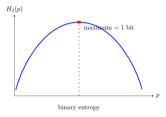
图 9 显示 Bernoulli variable 在 \(p=1/2\) 最不确定;\(p\to0\) 或 \(1\) 时 outcome 可预测,entropy 趋零。
communication channel 由 \(p(y\mid x)\) 定义。channel capacity 是对 input distribution 优化的 mutual information:
\[C=\max_{p(x)}I(X;Y).\]
它是 specified channel model 的可靠传输率上界,不是任意 network 的“带宽”。topological paths、physical noise、coding delay 与 resource cost 必须同时说明。
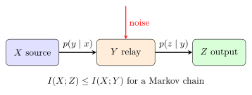
图 10 把 physical channel 与 information measure 分开:relay 可以 re-encode,却不能在 Markov assumption 下创造关于 \(X\) 的新信息。
Worked examples / 完整例题
Worked Example 1 — 小图的 degree、distance 与 clustering
已知: undirected graph 的 edges 为 \(AB,AC,BC,CD,DE\)。
研究对象与边界: 只把列出的五条边作为 \(E\);无 weights、self-loops 或 hidden edges。
参考系/坐标: graph 无空间坐标;只计 edge hops。
模型理由: 这是检验 K01 definitions 的最小非平凡图。
degrees 为
\[(k_A,k_B,k_C,k_D,k_E)=(2,2,3,2,1), \qquad \sum_i k_i=10=2M.\]
十个 unordered pairs 的 distances 依次为
\[1,1,2,3,1,2,3,1,2,1,\]
故
\[\ell=\frac{17}{10}=1.70.\]
\(A,B\) 的 neighbor pairs 已连接,故 \(C_A=C_B=1\);\(C\) 的三个 neighbors 中仅 \(AB\) 连边,故 \(C_C=1/3\);\(D\) 的 neighbors 未互连,\(C_D=0\);按本课 convention \(C_E=0\)。因此
\[\bar C=\frac{1+1+1/3}{5}=0.467.\]
单位/有效数字: degree、distance、clustering 都 dimensionless;\(\ell\) 与 \(\bar C\) 报三位有效数字。
检查: handshake lemma 通过;所有 pairs connected,未引入 infinite distance。
物理解释: triangle \(ABC\) 产生 local redundancy,但 bridge-like chain \(C-D-E\) 拉长 global paths。
Worked Example 2 — Erdős–Rényi degree 与 isolated vertices
已知: \(G(N,p)\) 中 \(N=1000\)、\(p=0.00600\)。
研究对象与边界: independent simple edges;不考虑 geometry、clustering mechanism 或 degree correlation。
参考系/坐标: 无空间坐标。
模型理由: 用 null model 估计平均 degree 与 isolated count。
\[\langle k\rangle=p(N-1) =(0.00600)(999)=5.994.\]
一个 vertex isolated 的 probability 是 \((1-p)^{N-1}\),所以
\[\mathbb E[N_0] =N(1-p)^{N-1} =1000(0.994)^{999} \approx2.45.\]
expected edges 为
\[\mathbb E[M] =p\binom{N}{2} =0.00600\frac{(1000)(999)}2 =2.997\times10^3.\]
单位/有效数字: counts dimensionless;expectation 可非整数,实际 realization 必为整数。
合理性检查: \(2\mathbb E[M]/N=5.994\) 与 \(\langle k\rangle\) 一致。
物理解释: mean degree 约 6 不保证每个 vertex connected;tail events 与 components 仍需 distribution-level analysis。
Worked Example 3 — configuration model 的 transmission threshold
已知: \(P(1)=0.20\)、\(P(2)=0.50\)、\(P(4)=0.30\);edge transmissibility \(\mathcal T=0.600\)。
研究对象与边界: large, uncorrelated, locally tree-like configuration network;SIR-to-bond-percolation mapping。
参考系/坐标: time 已吸收到 integrated transmissibility \(\mathcal T\)。
模型理由: degree moments 给出 early branching threshold。
\[\langle k\rangle =(0.20)(1)+(0.50)(2)+(0.30)(4) =2.40,\]
\[\langle k^2\rangle =(0.20)(1)+(0.50)(4)+(0.30)(16) =7.00.\]
于是
\[\mathcal T_c =\frac{2.40}{7.00-2.40} =0.522.\]
early excess-degree reproduction factor 是
\[\mathcal R_{\mathrm{edge}} =\mathcal T\frac{\langle k^2\rangle-\langle k\rangle}{\langle k\rangle} =(0.600)\frac{4.60}{2.40} =1.15>1.\]
单位/有效数字: probabilities and moments dimensionless;三位有效数字。
极限/方向检查: \(\mathcal T=0\) 时无传播;\(\mathcal R_{\mathrm{edge}}>1\) 表示 giant outbreak possible,不表示必然发生。
模型边界/解释: clustering、degree correlation、adaptive behavior 与 temporal contacts 会改变 threshold。
Worked Example 4 — binary symmetric channel 的信息率
已知: equiprobable bit \(X\) 通过 crossover probability \(\varepsilon=0.100\) 的 binary symmetric channel;求 \(I(X;Y)\)。
研究对象与边界: memoryless channel,每次 error independent;只算 per-symbol information。
参考系/符号: logarithm base 2;\(Y\ne X\) probability 为 \(\varepsilon\)。
模型理由: symmetry 使 uniform input 同时达到 channel capacity。
binary entropy 为
\[H_2(\varepsilon) =-\varepsilon\log_2\varepsilon -(1-\varepsilon)\log_2(1-\varepsilon) =0.469\ \mathrm{bit}.\]
uniform input 给 \(H(Y)=1\) bit,且 \(H(Y\mid X)=H_2(\varepsilon)\),所以
\[I(X;Y)=1-H_2(0.100)=0.531\ \mathrm{bit\ per\ use}.\]
单位/有效数字: information 用 bit,三位有效数字。
极限检查: \(\varepsilon\to0\) gives 1 bit;\(\varepsilon\to1/2\) gives 0 bit。
物理解释: raw channel 每次仍发送一个 binary symbol,但其中可靠地关于 input 的平均 information 少于一 bit;coding theorem 还需要 long blocks and error-control coding。
Lesson synthesis / 全课综合
处理 network-physics problem 可用以下 workflow:
- 定义 vertices、edges、direction、weight、time window 与 missing-data rule;
- 先做 structural audit:degree sum、components、paths、clustering 与 null model;
- 再写 dynamics:conserved diffusion、stochastic transmission、threshold response 或 capacity-limited flow;
- 指定 observable:mixing time、outbreak probability、giant component、service loss 或 mutual information;
- 指定 perturbation ensemble:random failure、targeted attack、parameter uncertainty 或 measurement noise;
- 用 model comparison 与 out-of-sample data 检查,不从一条 log–log 直线或一张漂亮 network layout 推断机制;
- 把 topological、dynamical 与 informational claims 分开,再说明它们如何耦合。
Formula-and-decision table / 公式与决策表
| Question | Relation | Use when | Main limitation |
|---|---|---|---|
| Degree audit? | \(k_i=\sum_jA_{ij}\), \(\sum_i k_i=2M\) | simple undirected graph | directed/weighted graphs need in/out/strength |
| Mean distance? | \(\ell=2\sum_{i<j}d(i,j)/[N(N-1)]\) | connected graph | disconnected pairs need declared convention |
| Local clustering? | \(C_i=2t_i/[k_i(k_i-1)]\) | undirected, \(k_i\ge2\) | average clustering differs from transitivity |
| ER mean degree? | \(\langle k\rangle=p(N-1)\) | independent-edge null model | no geometry/correlation/growth |
| Preferential attachment? | \(\Pi_i=k_i/\sum_jk_j\) | stated BA growth model | not proof that data are scale-free |
| Linear graph diffusion? | \(\dot{\mathbf x}=-\kappa L\mathbf x\) | symmetric conservative edge flux | nonlinear/directed transport differs |
| Percolation threshold? | \(\mathcal T_c=\langle k\rangle/(\langle k^2\rangle-\langle k\rangle)\) | large uncorrelated tree-like configuration model | clustering and temporal contacts alter it |
| Connectivity robustness? | \(S(q)=N_{\mathrm{giant}}(q)/N_0\) | specified removal rule | says nothing automatic about flow/service |
| Shannon uncertainty? | \(H=-\sum p\log_2p\) | specified discrete distribution | not semantic or thermodynamic entropy by default |
| Shared information? | \(I(X;Y)=H(X)-H(X\mid Y)\) | joint distribution known | dependence is not causation |
Model boundaries / 模型边界
- static graphs erase timing; temporal order can create or destroy feasible paths。
- simple graphs omit direction, weight, capacity, spatial cost and multilayer dependence。
- \(G(N,p)\) independence is a null assumption, not a realistic generator for every system。
- “small-world” needs both short path lengths and a clustering comparison to an explicit null model。
- power-law fit requires statistical comparison and finite-size treatment;“scale-free” is not visually certified。
- Laplacian diffusion assumes linear symmetric flux and conserved node quantity。
- percolation mapping assumes specified independent transmissibility and network ensemble。
- robustness is observable- and perturbation-specific;connectivity survival is not operational safety。
- linear controllability does not guarantee feasible nonlinear control under energy, saturation and observation limits。
- Shannon measures require a probability ensemble;one deterministic message has no unique entropy without a coding model。
Misconception clinic / 误区诊所
- “degree 最大的 vertex 一定最重要。” 不一定。betweenness、dynamical sensitivity、capacity 与 control objective 可给不同 ranking。
- “布局图上靠得近就是 path 短。” 错。除非 geometry 被编码为 weight,否则只数 edges。
- “short average path 就是 small-world。” 不够;还需 substantial clustering 与恰当 null comparison。
- “log–log 直线证明 scale-free。” 错。有限范围、cutoff 与 alternative heavy tails 必须比较。
- “传播率高于 threshold 就人人感染。” 错。只表示 giant outbreak becomes possible;seed、finite size 与 stochastic extinction 仍重要。
- “增加 edges 总会提高安全性。” 错。redundancy 可提高 connectivity,也可扩大 cascade pathways 或同步失效。
- “random-failure robustness 意味抗攻击。” 错。perturbation ensemble 不同。
- “mutual information 证明 \(X\) 导致 \(Y\)。” 错。它测 statistical dependence,不给 causal direction。
- “entropy 高代表内容更有意义。” 错。Shannon entropy 不评价 semantic value。
Practice and retrieval / 练习与检索
- [K01] 一个 simple undirected graph 的 degrees 为 \((3,3,2,2,2)\)。它可能存在吗?若存在,edge count 为多少?
Answer 1
degree sum \(=12\) 为偶数,handshake lemma 给 \(M=12/2=6\);该序列可图化,例如先连接两个 degree-3 vertices,再分配其余 edges。偶数只是必要条件,完整判断可用 Havel–Hakimi。
- [K01] vertex \(i\) 有 5 个 neighbors,其中彼此有 4 条 edges。求 \(C_i\)。
Answer 2
possible neighbor pairs 为 \(\binom52=10\),所以 \(C_i=4/10=0.400\),等价于 \(2t_i/[k_i(k_i-1)]=8/20\)。
- [K02] \(G(500,0.0200)\) 的 expected degree 与 expected edge count 各是多少?
Answer 3
\(\langle k\rangle=(499)(0.0200)=9.98\);\(\mathbb E[M]=0.0200(500)(499)/2=2495\)。检查 \(2M/N=9.98\)。
- [K02] 某网络 \(\ell\) 与 size-matched random graph 相近,但 clustering 也与 random graph 相近。能否据此称为 Watts–Strogatz-type small-world?
Answer 4
证据不足。short paths 只满足一半特征;需要显著高于 null 的 clustering,并说明 size、degree distribution 与 sampling 一致。也不能由此声称 power law。
- [K03] 两节点以一条 edge 相连,\(\dot x_1=-\kappa(x_1-x_2)\)、\(\dot x_2=-\kappa(x_2-x_1)\)。difference \(\Delta=x_1-x_2\) 怎样衰减?
Answer 5
\(\dot\Delta=-2\kappa\Delta\),故 \(\Delta(t)=\Delta(0)e^{-2\kappa t}\);sum \(x_1+x_2\) conserved。mixing timescale 是 \((2\kappa)^{-1}\)。
- [K03] regular network degree \(k=4\) 的 locally tree-like approximation 给出怎样的 bond-percolation threshold?
Answer 6
\(\langle k\rangle=4\)、\(\langle k^2\rangle=16\),故 \(\mathcal T_c=4/(16-4)=1/3\)。真实二维 square lattice 有 loops,不能用此 tree-like value 替代其实际 threshold。
- [K04] 为什么只报告“删除 20% vertices 后仍有 giant component”不能证明电网服务可靠?
Answer 7
connectivity 不包含 power-flow equations、line capacities、frequency/voltage stability、generation-load balance 与 protection logic。必须定义 service observable 和 failure ensemble。
- [K04] 给定一条 line 初始 load \(80\ \mathrm{MW}\)、capacity \(100\ \mathrm{MW}\);neighbor failure 使其 load 增加 \(30\%\)。是否触发 overload?
Answer 8
new load \(=80(1.30)=104\ \mathrm{MW}>100\ \mathrm{MW}\),在 hard-threshold toy model 中 overload。真实设备有 thermal time constant、emergency rating 与 protection delay。
- [K05] Bernoulli variable 的 \(p=0.25\),求 entropy。
Answer 9
\(H_2(0.25)=-0.25\log_2 0.25-0.75\log_2 0.75=0.811\ \mathrm{bit}\),小于 fair bit 的 1 bit。
- [K05 综合] 若 \(Y=X\) deterministically 且 \(H(X)=2.00\) bit,求 \(H(Y\mid X)\) 与 \(I(X;Y)\);若再经独立 noise 得到 \(Z\),能否有 \(I(X;Z)>2.00\) bit?
Answer 10
\(H(Y\mid X)=0\),\(I(X;Y)=H(X)=2.00\) bit。Markov chain \(X\to Y\to Z\) 满足 data-processing inequality,所以 \(I(X;Z)\le2.00\) bit;独立 noise 不会增加关于 \(X\) 的信息。
Exit ticket / 迁移检验
某团队声称:“我们的 communication network 呈 scale-free,因此能快速扩散信息、抗随机故障,并且只需控制最大的 hub 就能稳定整个系统。”写出一份最少五项的证据清单,判断这段话哪些部分需要分别验证。
Exit-ticket benchmark
应分别要求:degree-tail 的 alternative-fit/cutoff test;path/clustering 与 matched null comparison;明确定义的信息动力学和传播时延;random 与 targeted removal 下的 service observable;capacity cascade model;明确的 state equation、actuator \(B\)、measurement 与 control objective;最后以 out-of-sample failure/communication data 验证。topology、dynamics、robustness 与 controllability 不能由同一个 “scale-free” 标签推出。
References and source notes / 参考资料与使用说明
以下权威直接来源均在 2026-08-31 实际打开并核对。正文重新组织,全部图依据方程原创绘制;未复制来源插图。
- MIT OpenCourseWare, 14.15J Networks — Lecture and Recitation Notes — graph metrics、random graphs、graph dynamics、diffusion and contagion 的课程结构。
- Watts, D. J. and Strogatz, S. H., Nature, Collective dynamics of small-world networks — rewiring model、high clustering 与 short characteristic path length。
- Barabási, A.-L. and Albert, R., arXiv/Science record, Emergence of scaling in random networks — growth plus preferential attachment 的原始模型与 journal DOI。
- MIT OpenCourseWare, 12.086 Modeling Environmental Complexity — Lecture Notes — percolation theory、random and scale-free networks 的本科建模边界。
- Newman, M. E. J., Physical Review E, Spread of epidemic disease on networks — SIR、transmissibility 与 bond-percolation mapping。
- Albert, R., Jeong, H. and Barabási, A.-L., Nature, Error and attack tolerance of complex networks — random failure 与 targeted removal 的不同 robustness response。
- Shannon, C. E., Bell System Technical Journal / IEEE, A Mathematical Theory of Communication — entropy、mutual information 与 channel-capacity framework 的原始来源。
- Clauset, A., Shalizi, C. R. and Newman, M. E. J., SIAM Review, Power-Law Distributions in Empirical Data — maximum-likelihood fitting、goodness-of-fit、alternative comparison 与 power-law range 的经验检验协议。
- Motter, A. E. and Lai, Y.-C., Physical Review E, Cascade-based attacks on complex networks — load redistribution、capacity exceedance 与 overload cascade 的原始模型。
- Liu, Y.-Y., Slotine, J.-J. and Barabási, A.-L., Nature, Controllability of complex networks — linear structural controllability、maximum matching 与 driver-node framework。
- MIT OpenCourseWare, 6.441 Information Theory — Lecture Notes — information measures、mutual-information identities、Markov chains 与 data-processing inequality。
Source-to-content map
| Source | Used for | Knowledge ID / Section | Model boundary or convention |
|---|---|---|---|
| MIT OCW 14.15J | graph representations, metrics, dynamics and diffusion | K01, K02, K03 | course framework; equations here use stated undirected conventions |
| Watts–Strogatz 1998 | small-world rewiring, clustering and path length | K02 | model is not a universal classifier of empirical networks |
| Barabási–Albert 1999 | growth plus preferential attachment | K02 | generative model alone does not validate an empirical power law |
| Clauset–Shalizi–Newman 2009 | empirical power-law fit, goodness-of-fit and alternative comparison | K02 | a log--log line is insufficient; finite range and sampling must be tested |
| MIT OCW 12.086 | percolation and random/scale-free model hierarchy | K02, K03 | selected analytic thresholds require specified ensembles |
| Newman 2002 | SIR–bond-percolation mapping | K03 | locally tree-like and transmission assumptions stated |
| Albert–Jeong–Barabási 2000 | random failure versus targeted attack | K04 | robustness metric and perturbation rule must be specified |
| Motter–Lai 2002 | load redistribution and overload cascades | K04 | capacity/load dynamics must be stated; topology alone is insufficient |
| Liu–Slotine–Barabási 2011 | driver nodes in linear structural controllability | K04 | does not establish feasible control of constrained nonlinear dynamics |
| Shannon 1948 | entropy, conditional entropy, mutual information, capacity | K05 | base-2 convention; semantic content and causality excluded |
| MIT OCW 6.441 | information identities, Markov chains and data-processing inequality | K05 | claims require the stated joint/channel model |
复习与拓展
- 下一课 Quantitative Decisions in Applied Physics 将把 network observables、uncertainty 与 evidence communication 放入具体决策边界。
- 可扩展:directed/weighted/multilayer/temporal networks、centrality、community detection、spectral sparsification、graph neural dynamics、causal inference 与 transfer entropy。
- 与 Emergence and Collective Dynamics 的接口:同一 local rule 在不同 \(A\) 上可出现不同 macroscopic phase;本课提供结构与信息层的诊断量。