
Learning objectives / 学习目标
完成本课后,你应当能够:
- 用“无净热传递”定义热平衡,并用第零定律说明温度计为什么可行。
- 区分经验温标、热力学温度与 ITS-90 实用温标,正确转换 K、°C 与 °F。
- 说明 2019 年后 kelvin 由精确的 Boltzmann 常数定义;水三相点不再定义 kelvin。
- 建立测温属性与温度之间的校准关系,评价灵敏度、量程、线性、响应时间与扰动。
- 从线膨胀推导面积与体膨胀,计算自由膨胀、热应力及液体表观膨胀。
- 识别小温差、各向同性、系数近似恒定等模型边界。
Prerequisites / 先修知识
- 能量传递与机械平衡的基本概念;
- 一次函数、图像斜率、初等代数与简单导数;
- 能用系统边界区分“系统本身的状态”与“跨边界的过程”。
Scope and conventions / 范围与约定
全篇使用 SI。温度本身用 \(T\)(K),Celsius 温度用 \(t\)(\(^\circ\mathrm C\)),温差写 \(\Delta T\)。因为 \(1\ \mathrm K\) 与 \(1\ ^\circ\mathrm C\) 的间隔相等,温差数值可以相同,但绝对温度不能混用 K 与 \(^\circ\mathrm C\)。除特别说明,物体均足够接近内部热平衡,可由单一温度描述;非平衡统计温度、极低温实现学与相对论温度不在本课范围。
Notation and modeling contract / 符号与建模契约
| Symbol | Meaning | SI unit / convention |
|---|---|---|
| \(T\) | thermodynamic temperature / 热力学温度 | K,必须为绝对温度 |
| \(t\) | Celsius temperature / 摄氏温度 | \(^\circ\mathrm C\) |
| \(X\) | thermometric property / 测温属性 | 随传感器而定 |
| \(\alpha,\beta\) | 线膨胀、体膨胀系数 | \(\mathrm{K^{-1}}\) |
| \(Q\) | 因温差跨系统边界的能量 | J;不是系统“含有”的量 |
标量温度不携带方向;\(\Delta T\) 的正负由末态减初态定义。膨胀公式默认小应变、材料均匀且系数在所考察温区近似恒定。
0. Before starting: four different statements
| Statement | Physical meaning | Typical test |
|---|---|---|
| \(T_A>T_B\) | A 的热力学温度较高 | 允许热接触后能量净流向 B |
| \(T_A=T_B\) | A、B 处于互相热平衡 | 宏观状态不再因热接触而变 |
| \(Q>0\) | 约定的系统在某过程中因温差获得能量 | 需要先画系统边界 |
| \(U_A>U_B\) | A 的内能更大 | 不能仅由温度大小推出 |
温度是状态量(state variable);热量 \(Q\) 是跨过系统边界的过程量(process quantity)。后者将在下一课系统展开。
Knowledge 1 — Thermal equilibrium and the zeroth law / 热平衡与热力学第零定律
Knowledge ID: P03-U01-L01-K01
1.1 Thermal contact and thermal equilibrium
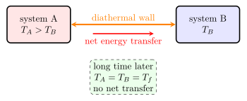
若两个系统之间的边界允许由温差驱动的能量传递,该边界称为透热壁(diathermal wall);理想地阻止这种传递的边界称为绝热壁(adiabatic wall)。
把 A 与 B 置于热接触后,若所有可观测宏观量不再随时间作系统性变化,并且两者之间没有净热传递,则称
\[\boxed{A\sim_{\rm th}B}\]
即 A 与 B 处于热平衡。微观能量交换仍可能双向发生;“平衡”要求的是统计平均的净交换为零,不是粒子停止运动。1
1.2 The zeroth law is a transitivity principle
热力学第零定律(zeroth law):
若 A 与 C 分别处于热平衡,且 B 与 C 也处于热平衡,则 A 与 B 处于热平衡。
符号化为
\[A\sim_{\rm th}C,\qquad B\sim_{\rm th}C \quad\Longrightarrow\quad A\sim_{\rm th}B.\]
把热平衡视为具有自反性、对称性和传递性的等价关系时,它把平衡态划分为一组组等温类;再用可排序的标量温度 \(T\) 标记这些类,使
\[A\sim_{\rm th}B \quad\Longleftrightarrow\quad T_A=T_B.\]
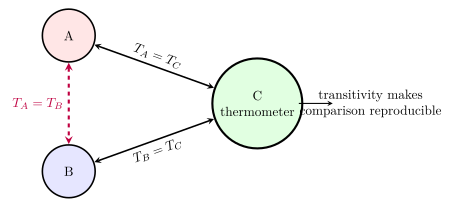
C 就是温度计。它不需要让 A 和 B 直接接触,却能给它们可比较的读数。
1.3 Equilibrium is conditional, not instantaneous
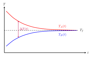
物体达到热平衡需要有限时间。一个简单的集总模型给出
\[T_A(t)-T_B(t)\propto e^{-t/\tau},\]
其中 \(\tau\) 是由热容与热耦合共同决定的时间尺度。若物体内部温度梯度很大,就不能用单一 \(T_A(t)\) 描述;那是传热课中的分布参数问题。
Knowledge 2 — Empirical and absolute temperature scales / 经验温标与绝对温标
Knowledge ID: P03-U01-L01-K02
2.1 An empirical scale is a calibrated ordering
选定一个随冷热程度单调变化的测温属性 \(X\),再规定函数
\[t=f(X).\]
这就建立了经验温标(empirical temperature scale)。若只用两个固定点并假设线性,
\[t=t_1+(t_2-t_1)\frac{X-X_1}{X_2-X_1}.\]
不同的 \(X\) 可能在固定点之间给出略有差别的读数;经验温标不是自动等于热力学温标。
2.2 Celsius, Fahrenheit, and kelvin
现行 SI 中,Celsius 温度由 kelvin 温度定义:
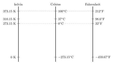
\[\boxed{t/^\circ\mathrm C=T/\mathrm K-273.15}.\]
Fahrenheit 与 Celsius 的精确线性换算为
\[\boxed{t_F=\frac95t_C+32}, \qquad \boxed{t_C=\frac59(t_F-32)}.\]
2.3 Absolute temperature and the 2019 kelvin
热力学温度的零点是绝对零度。2019 年 5 月 20 日起,kelvin 的大小通过给 Boltzmann 常数固定精确值来定义:
\[\boxed{k_B=1.380\,649\times10^{-23}\ \mathrm{J\,K^{-1}}\quad\text{exact}}.\]
因此 \(k_BT\) 把温度尺度与能量尺度连接起来。现在水三相点不再定义 kelvin;它仍是高度可复现的校准状态,并在 ITS-90 上赋值 \(273.16\ \mathrm K\)。234
2.4 Constant-volume gas thermometer: an operational bridge
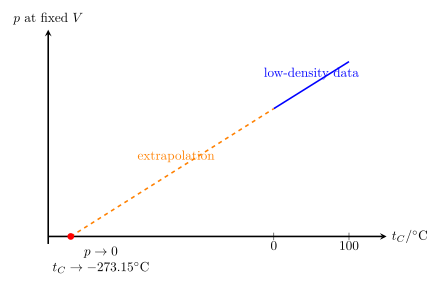
稀薄气体在定容下近似满足 \(p\propto T\)。对多种低密度气体,把 \(p\)–\(t_C\) 直线外推到 \(p=0\),截距趋向 \(-273.15^\circ\mathrm C\)。这不是“真的把经典气体冷到零压”,而是低密度极限的外推;真实气体会先凝结,量子效应也会在低温出现。
2.5 Worked Example 1 — scale conversion
某烘箱读数为 \(425^\circ\mathrm F\)。求 Celsius 与 kelvin 温度。
已知条件: \(t_F=425^\circ\mathrm F\);原读数分辨率为 \(1^\circ\mathrm F\)。
研究对象: 烘箱处于该读数时的温度状态。
系统边界 / 参考系: 只做同一温度状态在不同标度间的换算,不讨论烘箱与环境之间的能量交换;空间参考系不参与计算。
坐标与正方向: N/A。温标换算是仿射映射,不是空间矢量;只约定更高读数代表更高温度。
模型及理由: 使用 Fahrenheit、Celsius 与 kelvin 的定义关系。温标零点不同,因此先处理偏置再处理刻度比例。
方程建立:
\[\frac{t_C}{^\circ\mathrm C} =\frac59\left(\frac{t_F}{^\circ\mathrm F}-32\right), \qquad \frac{T}{\mathrm K} =\frac{t_C}{^\circ\mathrm C}+273.15.\]
比值 \(t_C/^\circ\mathrm C\)、\(t_F/^\circ\mathrm F\) 与 \(T/\mathrm K\) 都是对应温标的数值,因此等式两边无量纲一致。
逐步计算:
\[t_C=\frac59(425-32)=218.3^\circ\mathrm C,\]
\[T=218.3+273.15=491.5\ \mathrm K.\]
SI 与有效数字: kelvin 是 SI 热力学温度单位。\(1^\circ\mathrm F\) 对应 \(5/9^\circ\mathrm C\approx0.6^\circ\mathrm C\),因此报告到 \(0.1^\circ\mathrm C\) 或 \(0.1\ \mathrm K\) 已足够,得到 \(218.3^\circ\mathrm C\) 与 \(491.5\ \mathrm K\)。
方向 / 量纲检查: \(425^\circ\mathrm F\) 明显高于水的标准沸点 \(212^\circ\mathrm F\),故 \(t_C>100^\circ\mathrm C\) 合理;kelvin 数值必须为正,且 Celsius 与 kelvin 的温差数值相同。
极限或合理性检查: 代入 \(32^\circ\mathrm F\) 会得到 \(0^\circ\mathrm C\),代入 \(212^\circ\mathrm F\) 会得到 \(100^\circ\mathrm C\),验证线性关系及偏置无误。
物理解释: 三个数值描述同一热状态,而非三个不同温度。辐射定律或理想气体公式必须使用 \(491.5\ \mathrm K\),不能把 \(218.3\) 当作绝对温度代入。
Knowledge 3 — Thermometers and thermometric properties / 温度计与测温属性
Knowledge ID: P03-U01-L01-K03
3.1 Measurement is comparison plus calibration
可用作温度计的属性包括液柱体积、电阻、热电势、气体压强、声速与辐射谱。它们必须满足:
- 在目标量程内与 \(T\) 有稳定、最好单调的关系;
- 可重复校准,且漂移与滞后可控;
- 传感器与被测物达到足够接近的热平衡;
- 传感器热容和接触方式不会显著改变被测温度。
3.2 Linear calibration and its residual
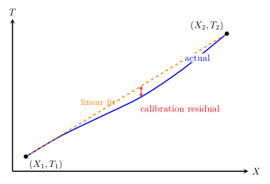
两点线性校准写成
\[T_{\rm lin}(X)=T_1+\frac{T_2-T_1}{X_2-X_1}(X-X_1).\]
真实关系若含曲率,
\[T(X)=a+bX+cX^2+\cdots,\]
两固定点处误差可以为零,中间仍存在非线性残差(nonlinearity residual)。
局部灵敏度为
\[S_X=\frac{dX}{dT}.\]
读出分辨率 \(\delta X\) 对应的理想温度分辨率近似为
\[\delta T\approx\frac{\delta X}{\lvert S_X\rvert}.\]
3.3 Dynamic response and loading
把小传感器近似为温度均匀的集总热容,置于恒温环境 \(T_\infty\) 中:
\[C_{\rm th}\frac{dT_s}{dt}=G(T_\infty-T_s),\]
解为
\[\boxed{T_s(t)=T_\infty+[T_s(0)-T_\infty]e^{-t/\tau}}, \qquad \tau=\frac{C_{\rm th}}{G}.\]
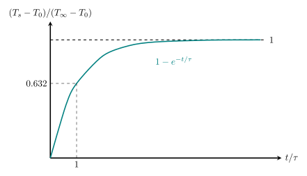
一个时间常数后完成最终变化的 \(63.2\%\),约 \(5\tau\) 后达到 \(99.3\%\)。若被测物本身很小,传感器的热容会把其温度拉向传感器初温,这叫loading error。
3.4 Contact and non-contact thermometry
| Type | Strength | Principal limitation |
|---|---|---|
| 液体玻璃温度计 | 直观、无需电源 | 量程、响应慢、浸没误差 |
| 电阻温度计 | 稳定、可高精度校准 | 自热、导线电阻、接触 |
| 热电偶 | 量程宽、结点小 | 需参考端补偿,输出小 |
| 红外温度计 | 非接触、响应快 | 依赖发射率、视场和窗口透射 |
3.5 Worked Example 2 — resistance thermometer
某电阻温度计在 \(0.00^\circ\mathrm C\) 与 \(100.00^\circ\mathrm C\) 时分别读出 \(100.00\ \Omega\) 与 \(138.50\ \Omega\)。若假定线性,求读数 \(119.25\ \Omega\) 对应的温度。
已知条件: \((t_1,R_1)=(0.00^\circ\mathrm C,100.00\ \Omega)\)、\((t_2,R_2)=(100.00^\circ\mathrm C,138.50\ \Omega)\),待测电阻 \(R=119.25\ \Omega\)。
研究对象: 与被测物达到热平衡后的电阻温度计感温元件。
系统边界 / 参考系: 把感温电阻及其两点校准关系作为测量系统;忽略导线电阻、自热、接触温差与响应滞后。空间参考系不参与计算。
坐标与正方向: N/A。把电阻随温度增大的方向规定为正;本校准区间内 \(R_2>R_1\),因此映射单调。
模型及理由: 题目明确要求在 \(0\)–\(100^\circ\mathrm C\) 内采用线性插值,故以两校准点唯一确定直线。该模型只在校准区间及仪器线性误差允许时成立。
方程建立: 一般的两点线性插值为
\[t=t_1+(t_2-t_1)\frac{R-R_1}{R_2-R_1}.\]
逐步计算: 待测电阻恰位于两校准电阻的中点:
\[\frac{R-R_1}{R_2-R_1} =\frac{119.25-100.00}{138.50-100.00} =0.5000.\]
因此
\[t_C=0.00^\circ\mathrm C +(100.00^\circ\mathrm C-0.00^\circ\mathrm C) \frac{119.25-100.00}{138.50-100.00} =50.00^\circ\mathrm C.\]
SI 与有效数字: 电阻比无量纲,结果单位继承为 \(^\circ\mathrm C\)。输入均给至 \(0.01\),在线性模型下报告 \(50.00^\circ\mathrm C\) 与给定精度一致。
方向 / 量纲检查: \(R_1<R<R_2\),所以必有 \(t_1<t<t_2\);算得 \(50.00^\circ\mathrm C\) 满足这一顺序。式中只能出现相同单位的电阻差之比。
极限或合理性检查: 若 \(R=R_1\),公式返回 \(t_1\);若 \(R=R_2\),返回 \(t_2\)。本题的中点电阻返回中点温度,是最直接的对称性检查。
物理解释: \(50.00^\circ\mathrm C\) 是在所选线性校准模型下的温度估计;若真实 \(R(T)\) 有二次项,两点校准不能消除中点误差,精确显示位数不等于真实准确度。
Knowledge 4 — Thermal expansion of solids and liquids / 固体与液体热膨胀
Knowledge ID: P03-U01-L01-K04
4.1 Linear expansion
各向同性固体的一条长度满足
\[\alpha(T)\equiv\frac1L \left(\frac{\partial L}{\partial T}\right)_{\sigma_{\rm ext}},\]
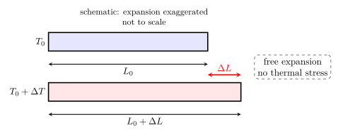
即在指定外应力(通常取无额外机械约束、近似零外应力)的自由膨胀条件下定义;受约束构件不能直接把这一定义式当作实际伸长。
若 \(\alpha\) 在温区内近似恒定,
\[\boxed{\Delta L=\alpha L_0\Delta T}, \qquad L\approx L_0(1+\alpha\Delta T).\]
更一般地,
\[\ln\frac{L_2}{L_1}=\int_{T_1}^{T_2}\alpha(T)\,dT.\]
4.2 Area and volume expansion
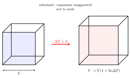
对各向同性固体,令原立方体边长为 \(L\):
\[V=L^3 \quad\Longrightarrow\quad \frac{dV}{V}=3\frac{dL}{L}.\]
因此小形变下
\[\boxed{\beta=3\alpha}, \qquad \boxed{\Delta V=\beta V_0\Delta T}.\]
面积系数相应为 \(2\alpha\)。这些关系不适用于各向异性晶体的所有方向;那时膨胀系数是张量。
4.3 Constraint creates thermal stress
自由热应变为
\[\varepsilon_{\rm th}=\alpha\Delta T.\]
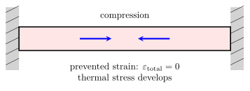
若一维杆被刚性支座完全阻止伸长,总应变为零,线弹性近似给出应力大小
\[\boxed{\lvert\sigma_{\rm th}\rvert=Y\alpha\lvert\Delta T\rvert}.\]
升温且被限制时通常产生压应力;降温且被限制时产生拉应力。公式要求材料仍在线弹性范围,支座近似刚性,温度均匀。
4.4 Liquids: real versus apparent volume expansion
液体没有独立于容器形状的“线膨胀”,通常定义体膨胀系数
\[\beta_\ell=\frac1V\left(\frac{\partial V}{\partial T}\right)_p.\]
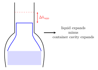
若液体装在会膨胀的容器中,观察到的液面变化对应表观体膨胀系数
\[\boxed{\beta_{\rm app}\approx\beta_\ell-\beta_c},\]
其中 \(\beta_c\) 是容器内腔的体膨胀系数。绝不能把液面上升直接等同于液体的真实膨胀。
4.5 Water anomaly
常压液态水在约 \(4^\circ\mathrm C\) 附近密度最大。把水从 \(0^\circ\mathrm C\) 加热到约 \(4^\circ\mathrm C\) 时,它反而收缩;因此该区间的有效 \(\beta\) 为负。这是“多数物质升温膨胀”的重要例外,不应使用恒定正 \(\beta\) 跨越该区间。IAPWS 给出常压水密度的精密关联式。5
4.6 Worked Example 3 — rail expansion
一根 \(L_0=30.0\ \mathrm m\) 的钢轨,\(\alpha=11.7\times10^{-6}\ \mathrm{K^{-1}}\),温度升高 \(55.0\ \mathrm K\)。求自由伸长量。
已知条件: \(L_0=30.0\ \mathrm m\)、\(\alpha=11.7\times10^{-6}\ \mathrm{K^{-1}}\)、\(\Delta T=+55.0\ \mathrm K\)。
研究对象: 一根可自由伸缩的均匀钢轨。
系统边界 / 参考系: 取整根钢轨为系统,在地面实验室参考系中比较加热前后长度;端部无约束,故不产生热应力。
坐标与正方向: 沿钢轨建立 \(+x\) 轴,正伸长定义为 \(\Delta L=L-L_0>0\)。
模型及理由: 温升均匀,\(\alpha\) 在该温区近似常数,且 \(\alpha\Delta T\ll1\),所以使用一阶线膨胀模型 \(\Delta L=\alpha L_0\Delta T\)。
方程建立:
\[L=L_0(1+\alpha\Delta T), \qquad \Delta L=\alpha L_0\Delta T.\]
逐步计算:
\[\Delta L=(11.7\times10^{-6})(30.0)(55.0) =1.93\times10^{-2}\ \mathrm m =1.93\ \mathrm{cm}.\]
SI 与有效数字: \(\mathrm{K^{-1}}\cdot\mathrm m\cdot\mathrm K=\mathrm m\);三个输入均为三位有效数字,故报告 \(1.93\times10^{-2}\ \mathrm m\)。
方向 / 量纲检查: \(\alpha>0\) 且 \(\Delta T>0\),所以 \(\Delta L>0\),即末端沿 \(+x\) 方向移动;正负号与“升温伸长”一致。
极限或合理性检查: \(\alpha\Delta T=6.44\times10^{-4}\ll1\),一阶近似合理;当 \(\alpha\to0\) 或 \(\Delta T\to0\) 时,\(\Delta L\to0\)。
物理解释: 约 \(1.93\ \mathrm{cm}\) 是整段 \(30.0\ \mathrm m\) 钢轨的自由长度变化。伸缩缝设计必须考虑可连续伸长的总长度,而不是只看单位长度。
4.7 Worked Example 4 — apparent liquid expansion
\(1.000\ \mathrm L\) 液体装满玻璃容器。取 \(\beta_\ell=1.10\times10^{-3}\ \mathrm{K^{-1}}\)、\(\beta_c=27.0\times10^{-6}\ \mathrm{K^{-1}}\),升温 \(40.0\ \mathrm K\)。求溢出体积。
已知条件: \(V_0=1.000\ \mathrm L=1.000\times10^{-3}\ \mathrm{m^3}\)、\(\beta_\ell=1.10\times10^{-3}\ \mathrm{K^{-1}}\)、\(\beta_c=27.0\times10^{-6}\ \mathrm{K^{-1}}\)、\(\Delta T=+40.0\ \mathrm K\)。
研究对象: 液体与限定其体积的玻璃容器空腔。
系统边界 / 参考系: 把初始装满的液体和容器作为组合系统;比较液体真实增容与容器空腔增容,忽略蒸发、泄漏及温度梯度。空间参考系不影响体积差。
坐标与正方向: N/A。把流出容器的体积定义为正的 \(\Delta V_{\rm spill}\)。
模型及理由: 两种材料均匀升温、体膨胀系数近似常数,且 \(\beta\Delta T\ll1\),故分别用 \(\Delta V=\beta V_0\Delta T\);表观溢出量是液体增容减空腔增容。
方程建立:
\[\Delta V_\ell=\beta_\ell V_0\Delta T, \qquad \Delta V_c=\beta_c V_0\Delta T,\]
\[\Delta V_{\rm spill}=\Delta V_\ell-\Delta V_c =V_0(\beta_\ell-\beta_c)\Delta T.\]
逐步计算:
\[\Delta V_\ell =(1.000\ \mathrm L)(1.10\times10^{-3})(40.0) =44.0\ \mathrm{mL},\]
\[\Delta V_c =(1.000\ \mathrm L)(27.0\times10^{-6})(40.0) =1.08\ \mathrm{mL},\]
\[\Delta V_{\rm spill} =V_0(\beta_\ell-\beta_c)\Delta T =42.9\ \mathrm{mL}.\]
SI 与有效数字: 体积膨胀式的单位为 \(\mathrm{m^3}\);这里转为 \(\mathrm{mL}\) 便于解释。受 \(40.0\ \mathrm K\) 和系数精度限制,报告三位有效数字 \(42.9\ \mathrm{mL}\)。
方向 / 量纲检查: 因 \(\beta_\ell>\beta_c\) 且 \(\Delta T>0\),差值为正,确有液体溢出;若差值为负,则会在容器上方形成空隙而不是“负溢出”。
极限或合理性检查: 若 \(\beta_\ell=\beta_c\),则 \(\Delta V_{\rm spill}=0\);若容器完全不膨胀,结果应回到 \(44.0\ \mathrm{mL}\)。本题 \(\beta_\ell\Delta T=0.044\ll1\),一阶模型尚可用。
物理解释: 容器空腔也随温度增大,所以观察到的溢出量 \(42.9\ \mathrm{mL}\) 小于液体自身的真实增容 \(44.0\ \mathrm{mL}\)。
5. Lesson synthesis / 全课整合
5.1 Concept chain
\[\text{thermal contact} \longrightarrow \text{equilibrium relation} \longrightarrow \text{zeroth law} \longrightarrow \text{temperature scale} \longrightarrow \text{calibrated thermometer}.\]
温度改变后,物体尺寸也可能改变:
\[\Delta T \longrightarrow \begin{cases} \Delta L=\alpha L_0\Delta T,\\ \Delta V=\beta V_0\Delta T,\\ \sigma_{\rm th}\ \text{if constrained}. \end{cases}\]
Formula-and-decision table / 公式—决策表
| Topic | Equation | Boundary |
|---|---|---|
| Celsius–kelvin | \(T/\mathrm K=t/^\circ\mathrm C+273.15\) | 绝对温度换算 |
| Two-point calibration | \(T=T_1+(T_2-T_1)(X-X_1)/(X_2-X_1)\) | 假定线性 |
| Sensor response | \(T_s-T_\infty=[T_s(0)-T_\infty]e^{-t/\tau}\) | 集总、一阶耦合 |
| Linear expansion | \(\Delta L=\alpha L_0\Delta T\) | \(\alpha\) 近似恒定 |
| Volume expansion | \(\Delta V=\beta V_0\Delta T\) | 小形变 |
| Isotropic solid | \(\beta\approx3\alpha\) | 各向同性 |
| Fully constrained rod | \(\lvert\sigma\rvert=Y\alpha\lvert\Delta T\rvert\) | 线弹性、完全约束 |
| Apparent liquid expansion | \(\beta_{\rm app}\approx\beta_\ell-\beta_c\) | 同一温差、小膨胀 |
Model boundaries / 模型边界
- 热平衡是宏观统计描述;极小系统会有明显涨落。
- 温度只有在局域平衡足够好时才是清晰的局域状态量。
- 线性温标校准不能自动消除非线性、滞后、自热或接触误差。
- 膨胀系数随温度、相态与晶向变化;大温区应积分。
- \(\beta=3\alpha\) 只适用于各向同性小形变固体。
- 热应力公式不覆盖塑性、蠕变、屈曲、裂纹与非均匀温场。
6. Misconception clinic / 易错概念诊所
| Misconception | Correction |
|---|---|
| “同温”表示两个物体含有相同热量 | 温度是状态量;热量是传递中的能量,不是储存量 |
| 达到热平衡后微观交换停止 | 双向微观交换继续,但净交换为零 |
| 第零定律只是“热从高温流向低温” | 它陈述热平衡关系的传递性,使温度标量与温度计成为可能 |
| \(20^\circ\mathrm C=20\ \mathrm K\) | \(20^\circ\mathrm C=293.15\ \mathrm K\);只有温差大小可相同 |
| kelvin 仍由水三相点定义 | 2019 年后由精确 \(k_B\) 定义;三相点仍用于 ITS-90 与校准 |
| 两点校准保证全量程准确 | 中间可能存在非线性残差 |
| 金属板受热时孔会缩小 | 均匀自由膨胀时孔也扩大 |
| 液面上升量就是液体真实膨胀量 | 它是液体与容器内腔膨胀之差 |
| 所有液体升温都膨胀 | 常压水在 \(0\) 到约 \(4^\circ\mathrm C\) 反常收缩 |
7. Practice and retrieval / 练习与检索
A. Conceptual questions
- A 与 C 热平衡,B 与 C 热平衡。若把 A 与 B 接触,会发生什么宏观净热传递?
- 为什么温度计必须足够小、等待足够久,但又不能无限小?
- 说明“水三相点不再定义 kelvin”与“它仍是 ITS-90 固定点”并不矛盾。
- 为什么带孔圆环均匀受热时孔径增大?
- 为什么表观液体膨胀可能小于真实膨胀?
B. Quantitative questions
- 把 \(-40.0^\circ\mathrm C\) 换算为 K 与 °F。
- 某线性温度计在 \(0^\circ\mathrm C\)、\(100^\circ\mathrm C\) 时读数分别为 12.0 与 87.0。读数 49.5 对应多少 °C?
- 传感器时间常数为 \(8.0\ \mathrm s\)。温度阶跃后多久完成最终变化的 \(95.0\%\)?
- 铝杆长 \(2.00\ \mathrm m\),\(\alpha=23.0\times10^{-6}\ \mathrm{K^{-1}}\),升温 \(80.0\ \mathrm K\)。求自由伸长。
- 上题铝杆若被完全限制,取 \(Y=69.0\ \mathrm{GPa}\),求压应力大小;判断是否应直接把答案当作实际结构应力。
- \(500\ \mathrm{mL}\) 液体的 \(\beta_\ell=7.5\times10^{-4}\ \mathrm{K^{-1}}\),容器 \(\beta_c=2.7\times10^{-5}\ \mathrm{K^{-1}}\),升温 \(30\ \mathrm K\)。求表观体积增加。
Answer 1
理想情况下无宏观净热传递,因为第零定律给出 \(T_A=T_C=T_B\)。
Answer 2
小热容可减小 loading,等待可减小动态误差;但无限小会降低信号、增加涨落并可能失去机械可靠性。
Answer 3
定义规定单位大小;实用温标规定可复现的实现与插值。两者角色不同。
Answer 4
把孔想象成同材质填充,整体膨胀后移走填充物。
Answer 5
容器内腔也膨胀,读数约对应 \(\beta_\ell-\beta_c\)。
Answer 6
\(233.15\ \mathrm K\);\(-40.0^\circ\mathrm F\)。
Answer 7
\((49.5-12.0)/(87.0-12.0)\times100=50.0^\circ\mathrm C\)。
Answer 8
\(1-e^{-t/\tau}=0.95\),故 \(t=-\tau\ln 0.05=24.0\ \mathrm s\)。
Answer 9
\(\Delta L=3.68\times10^{-3}\ \mathrm m=3.68\ \mathrm{mm}\)。
Answer 10
\(\lvert\sigma\rvert=Y\alpha\Delta T=127\ \mathrm{MPa}\);实际值还受支座柔度、屈服、温度梯度和屈曲影响。
Answer 11
\(\Delta V_{\rm app}=500(7.5\times10^{-4}-2.7\times10^{-5})30=10.8\ \mathrm{mL}\)。
Exit ticket
用不超过四句话回答:第零定律、kelvin 定义、温度计校准与液体表观膨胀之间的逻辑关系是什么?
8. References and source notes / 参考资料与使用说明
8.1 Source-to-content map
| Source | Used for | Knowledge ID / Section | Model boundary or convention |
|---|---|---|---|
| OpenStax University Physics Vol. 2, §1.1 | thermal contact, equilibrium, zeroth-law teaching sequence | K01 | macroscopic equilibrium |
| OpenStax University Physics Vol. 2, §1.2 | empirical thermometry, gas thermometer, scale conversions | K02–K03 | historical definition wording is superseded by current BIPM/NIST SI |
| OpenStax University Physics Vol. 2, §1.3 | linear/volume expansion, holes, thermal stress | K04 | small strain and nearly constant coefficients |
| BIPM — SI base unit: kelvin | current SI definition and exact \(k_B\) | K02 | normative post-2019 definition |
| BIPM — SI Brochure, 9th ed. v4.01 | normative SI wording, kelvin and Celsius relation | K02 | SI unit convention |
| BIPM — Guide to the Realization of the ITS-90, Part 1 | practical-scale scope, fixed points, interpolation framework | K02–K03 | realization rather than unit definition |
| NIST — Kelvin: Present Realization | 2019 redefinition and continuing calibration role of the water triple point | K02–K03 | current realization practice |
| NIST — Kelvin: ITS-90 | practical temperature scale and fixed points | K02–K03 | ITS-90 interpolation |
| IAPWS — Water and the temperature scale | water triple point, ITS-90 distinction, water-property context | K02 | water-specific convention |
| IAPWS — Properties of liquid water at 0.1 MPa | density maximum and model caution for water | K04 | water anomaly near \(4\ ^\circ\mathrm C\) |
8.2 Source notes
以上来源均于 2026-08-24 实际打开核对。本课把 OpenStax 用作 HS→UG1 教学主线,把 BIPM/NIST 作为 SI 与测温学的规范来源,把 IAPWS 作为水性质的第一方国际数据来源。所有图均按本课方程原创绘制,不复刻来源插图。
8.3 Reading route
- 温度改变需要多少能量:Heat Capacity and Phase Change。
- 温差如何驱动空间能量输运:Heat Transfer。
- 温度与分子运动的联系:Ideal-Gas Model。