
Learning objectives / 学习目标
完成本课后,你应当能够:
- 从 Kirchhoff 回路方程推导串联 RC 的充电、放电电压、电荷和电流。
- 解释时间常数的单位与物理意义,并用 \(1-e^{-1}\)、\(e^{-1}\) 和 \(5\tau\) 作快速估计。
- 用电容电压连续性、直流终态开路和 Thevenin 等效求任意单电容网络的 \(v_C(0^+)\)、\(v_C(\infty)\) 与 \(\tau\)。
- 写出一阶完整响应,检验符号、初值、终值、斜率和能量守恒。
- 推导无源 RC 低通与高通滤波器的传递函数、截止频率、幅频极限和相位。
- 建模阈值定时器,判断何时必须考虑源内阻、负载、电容漏电与非理想开关。
Prerequisites / 先修知识
- Capacitance and Stored Energy:\(q=Cv_C\)、\(U_C=Cv_C^2/2\)。
- Circuit Analysis:KCL、KVL 与 Thevenin equivalent。
- 数学:\(dy/dt+ay=b\) 的分离变量或积分因子解;指数函数和复数相量的基础。
Scope and conventions / 范围与约定
- 采用 lumped-element(集总元件)模型;导线传播延迟相对 \(RC\) 可忽略。
- 电容 \(C\) 与电阻 \(R\) 取常数,除非明确说明非理想性。
- \(v_C\) 定义为电容上端对下端电势;电流 \(i_C\) 流入标有正电压的端子时,使用 passive sign convention:\(i_C=C\,dv_C/dt\)。
- 开关动作定义为 \(t=0\);\(0^-\) 与 \(0^+\) 分别代表开关前后无限接近的时刻。
- 直流终态指独立源恒定且经过足够长时间;不是所有随时间变化的电路都可把电容视为开路。
- 滤波器部分使用正弦稳态与理想零输出阻抗源;负载效应单独讨论。
Notation and modeling contract / 符号与建模契约
| Symbol | Meaning | SI unit |
|---|---|---|
| \(q\) | capacitor plate charge | C |
| \(C\) | capacitance | F |
| \(v_C\) | signed capacitor voltage | V |
| \(i_C=C\,dv_C/dt\) | current entering positive-voltage terminal | A |
| \(R_{\mathrm{th}}\) | resistance seen by the capacitor with independent sources deactivated | \(\Omega\) |
| \(V_f\) | final DC capacitor voltage | V |
| \(V_0\) | \(v_C(0^+)=v_C(0^-)\) | V |
| \(\tau=R_{\mathrm{th}}C\) | time constant | s |
| \(\omega\) | angular frequency | \(\mathrm{rad\,s^{-1}}\) |
| \(H(\mathrm i\omega)\) | output/input phasor ratio | dimensionless |
Knowledge 1 — Capacitor charging and discharging / 电容器充放电
Knowledge ID: P04-U05-L04-K01
1.1 The state variable and its continuity
理想电容的 constitutive relation 是
\[q=Cv_C, \qquad i_C=\frac{dq}{dt}=C\frac{dv_C}{dt}.\]
若有限电流在零时间内把 \(v_C\) 改变有限量,则积分给出
\[\Delta v_C=\frac{1}{C}\int_{0^-}^{0^+}i_C(t)\,dt=0.\]
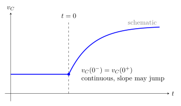
因此在没有理想冲激电流时,
\[\boxed{v_C(0^+)=v_C(0^-)}.\]
这不是“电容电压永远不变”,而是“不能跳变”;其后可以连续变化。
1.2 Charging from an ideal DC source
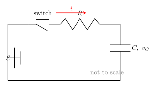
对未充电电容、理想电压源 \(\mathcal E\) 和电阻 \(R\) 的串联回路,令充电电流为正。KVL 给出
\[\mathcal E-iR-v_C=0, \qquad i=C\frac{dv_C}{dt}.\]
于是
\[RC\frac{dv_C}{dt}+v_C=\mathcal E.\]
由 \(v_C(0)=0\) 得
\[\boxed{v_C(t)=\mathcal E\left(1-e^{-t/(RC)}\right)},\]
\[\boxed{q(t)=C\mathcal E\left(1-e^{-t/(RC)}\right)}, \qquad \boxed{i(t)=\frac{\mathcal E}{R}e^{-t/(RC)}}.\]
1.3 Discharging through a resistor
若初值 \(v_C(0)=V_0\),移除电源后电容经 \(R\) 放电。仍定义 \(i_C\) 流入正端,则
\[Ri_C+v_C=0, \qquad RC\frac{dv_C}{dt}+v_C=0.\]
因此
\[\boxed{v_C(t)=V_0e^{-t/(RC)}}, \qquad \boxed{i_C(t)=-\frac{V_0}{R}e^{-t/(RC)}}.\]
负号表示实际放电电流流出电容正端。电容初始能量
\[U_0=\frac12CV_0^2\]
最终全部转化为电阻内能:
\[\int_0^\infty i^2R\,dt =\frac{V_0^2}{R}\int_0^\infty e^{-2t/(RC)}dt =\frac12CV_0^2.\]
Knowledge 2 — Time constant and exponential response / 时间常数与指数响应
Knowledge ID: P04-U05-L04-K02
2.1 General first-order response
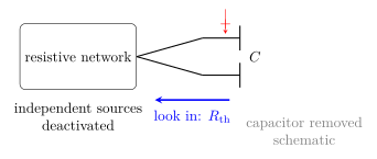
从电容端口向外看,任意线性电阻网络可化为 Thevenin voltage \(V_{\mathrm{th}}\) 与 \(R_{\mathrm{th}}\)。于是
\[R_{\mathrm{th}}C\frac{dv_C}{dt}+v_C=V_{\mathrm{th}}.\]
若源在 \(t>0\) 恒定,完整解为
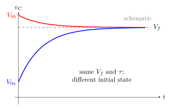
\[\boxed{v_C(t)=V_f+(V_0-V_f)e^{-t/\tau}}, \qquad \boxed{\tau=R_{\mathrm{th}}C},\]
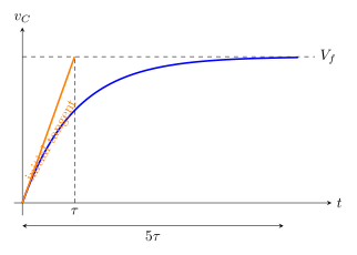
其中 \(V_0=v_C(0^+)\),\(V_f=v_C(\infty)=V_{\mathrm{th}}\)。偏离终值的量满足
\[\frac{v_C(t)-V_f}{V_0-V_f}=e^{-t/\tau}.\]
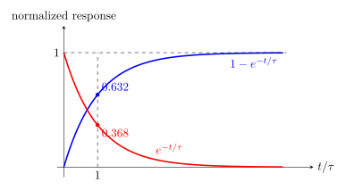
因此每经过一个 \(\tau\),剩余偏差乘以 \(e^{-1}\approx0.368\)。
2.2 Units, tangent interpretation, and five-time-constant rule
量纲检验:
\[[RC]=\frac{\mathrm V}{\mathrm A}\frac{\mathrm C}{\mathrm V} =\frac{\mathrm C}{\mathrm A}=\mathrm s.\]
初始斜率由微分方程直接给出:
\[\left.\frac{dv_C}{dt}\right|_{0^+}=\frac{V_f-V_0}{\tau}.\]
在 \(t=0\) 作切线,它与终值线相交于 \(t=\tau\)。在 \(5\tau\) 后,偏差为 \(e^{-5}=0.00674\),即完成 99.33%;“完全充满”只是工程近似,数学上只渐近达到。
2.3 Finding \(R_{\mathrm{th}}\)
断开电容,把独立电压源替换为短路、独立电流源替换为开路,然后从电容两端看进去求等效电阻。若含受控源,不能关闭受控源;应在端口加测试源,用 \(R_{\mathrm{th}}=V_{\mathrm{test}}/I_{\mathrm{test}}\)。
Knowledge 3 — Initial and final conditions / 初始与终态条件
Knowledge ID: P04-U05-L04-K03
3.1 The three-number method
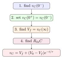
对只有一个独立储能元件的一阶 RC 网络,最可靠流程是:
- Before: 用 \(t<0\) 电路求 \(v_C(0^-)\);若已长期直流稳态,电容视为开路。
- Continuity: 若无冲激电流,\(v_C(0^+)=v_C(0^-)=V_0\)。
- After-final: 用 \(t>0\) 电路求 \(v_C(\infty)=V_f\);长期直流时电容开路。
- Resistance: 从电容端口求 \(R_{\mathrm{th}}\),进而 \(\tau=R_{\mathrm{th}}C\)。
- Assemble: \(v_C=V_f+(V_0-V_f)e^{-t/\tau}\)。
3.2 Immediate post-switch circuit is not a DC steady state
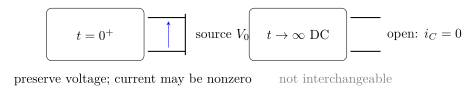
在 \(0^+\),可以把电容暂时等效为一个电压为 \(V_0\) 的理想电压源来求瞬时电流;只有当 \(V_0=0\) 时,这个瞬时等效才像短路。在 \(t\to\infty\) 的恒定源电路中,\(i_C\to0\),电容才像开路。
3.3 A built-in diagnostic: initial slope
得到候选解后,不仅检查两端点,还应检查
\[i_C(0^+)=C\left.\frac{dv_C}{dt}\right|_{0^+}=\frac{V_f-V_0}{R_{\mathrm{th}}}.\]
右式正负必须与 \(0^+\) 电路中实际电流方向一致。若 \(V_f>V_0\),电容电压上升;若 \(V_f<V_0\),下降;不存在无缘无故的过冲,因为单个无源 RC 一阶网络的响应单调。
Knowledge 4 — RC filters and timing applications / RC 滤波与定时应用
Knowledge ID: P04-U05-L04-K04
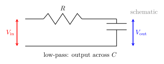
4.1 Low-pass: output across the capacitor
正弦稳态下,电容阻抗 \(Z_C=1/(\mathrm i\omega C)\)。串联 \(R\)、\(C\) 且输出取在 \(C\) 上:
\[\boxed{H_{\mathrm{LP}}(\mathrm i\omega) =\frac{V_{\mathrm{out}}}{V_{\mathrm{in}}} =\frac{1}{1+\mathrm i\omega RC}}.\]
\[\lvert H_{\mathrm{LP}}\rvert =\frac{1}{\sqrt{1+(\omega RC)^2}}, \qquad \phi_{\mathrm{LP}}=-\tan^{-1}(\omega RC).\]
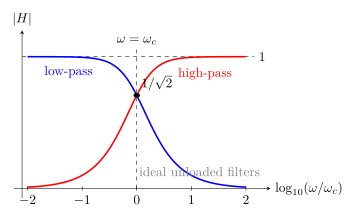
在 \(\omega_c=1/(RC)\),幅度为 \(1/\sqrt2\),功率比为 \(1/2\),即 \(-3.01\ \mathrm{dB}\)。
4.2 High-pass: output across the resistor
输出改取在 \(R\) 上:
\[\boxed{H_{\mathrm{HP}}(\mathrm i\omega) =\frac{\mathrm i\omega RC}{1+\mathrm i\omega RC}},\]
\[\lvert H_{\mathrm{HP}}\rvert =\frac{\omega RC}{\sqrt{1+(\omega RC)^2}}, \qquad \phi_{\mathrm{HP}}=\tan^{-1}\!\left(\frac{1}{\omega RC}\right).\]
低频时电容阻抗大,输出趋近零;高频时电容阻抗小,输出趋近输入。两者截止角频率相同。
4.3 Step response and timing threshold
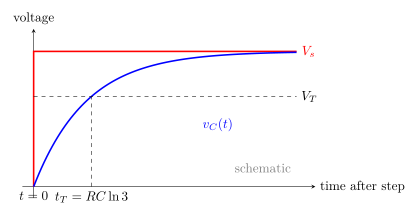
低通 RC 同时是 step-response circuit。对 \(0\to V_s\) 的阶跃,\(v_C=V_s(1-e^{-t/RC})\)。若比较器在 \(V_T\) 触发,且 \(0<V_T<V_s\),则
\[\boxed{t_T=-RC\ln\!\left(1-\frac{V_T}{V_s}\right)}.\]
4.4 Loading and nonideal boundaries
若输出端接有限负载 \(R_L\),低通网络的直流增益与时间常数都会改变;必须把 \(R_L\) 包含在电容所见网络中。实际电容还可能有 equivalent series resistance、漏电阻、容差和电压依赖。理想传递函数只在元件线性、频率低于寄生电感显著区且测量仪器负载可忽略时可靠。
Worked Examples / 完整例题
Worked Example 1 — A charging capacitor with sign and energy checks
Known. \(\mathcal E=12.0\ \mathrm V\),\(R=2.00\ \mathrm{k\Omega}\),\(C=150\ \mathrm{\mu F}\),初始未充电。求 \(t=0.450\ \mathrm s\) 的 \(v_C\)、\(i\)、\(q\) 与电阻瞬时功率。
Object, boundary, reference, direction. 研究对象是串联 \(R\)–\(C\) 回路;源、\(R\)、\(C\) 均在系统内。令充电电流从源正端经 \(R\) 流向电容正端为正,\(t=0\) 合闸。
Model and reason. 理想恒压源、线性 \(R,C\),单一储能元件,故用一阶充电模型。
Equations and calculation.
\[\tau=RC=(2.00\times10^3)(150\times10^{-6})=0.300\ \mathrm s,\]
\[e^{-t/\tau}=e^{-1.50}=0.22313.\]
\[v_C=12.0(1-0.22313)=9.32\ \mathrm V,\]
\[i=\frac{12.0}{2000}(0.22313)=1.34\times10^{-3}\ \mathrm A,\]
\[q=Cv_C=(150\times10^{-6})(9.32)=1.40\times10^{-3}\ \mathrm C,\]
\[P_R=i^2R=(1.34\times10^{-3})^2(2000)=3.58\times10^{-3}\ \mathrm W.\]
Checks and interpretation. \(v_C<12.0\ \mathrm V\)、\(i>0\) 且随时间下降;KVL 检查 \(iR+v_C=2.68+9.32=12.00\ \mathrm V\)。三位有效数字合理;\(RC\) 的单位为秒。
Worked Example 2 — Discharge time and recovered energy
Known. \(C=47.0\ \mathrm{\mu F}\) 先充到 \(V_0=30.0\ \mathrm V\),后经 \(R=330\ \mathrm{k\Omega}\) 放电。求降至 \(5.00\ \mathrm V\) 的时间以及这段期间电阻吸收的能量。
Object and convention. 电容和电阻组成孤立系统;\(v_C\) 初始正端不变,实际放电电流流出正端。参考时刻为接通电阻瞬间。
Model. 漏电和 ESR 忽略,\(R,C\) 线性。
\[\tau=RC=(330\times10^3)(47.0\times10^{-6})=15.51\ \mathrm s.\]
由 \(5.00=30.0e^{-t/\tau}\):
\[t=\tau\ln\frac{30.0}{5.00}=15.51\ln 6=27.8\ \mathrm s.\]
能量账本给出
\[\Delta E_R=\frac12C(V_0^2-V^2) =\frac12(47.0\times10^{-6})(30.0^2-5.00^2) =2.06\times10^{-2}\ \mathrm J.\]
Checks. 电压比无量纲;\(t=1.79\tau\) 对应 \(e^{-1.79}\approx1/6\)。能量为正且小于初始 \(0.0212\ \mathrm J\),符合守恒。
Worked Example 3 — Switched network via Thevenin reduction
Known. 开关前电容已长期接在 \(9.00\ \mathrm V\) 理想源上。\(t=0\) 后,\(C=20.0\ \mathrm{\mu F}\) 接到由 \(12.0\ \mathrm V\) 源、\(R_1=4.00\ \mathrm{k\Omega}\) 上臂、\(R_2=6.00\ \mathrm{k\Omega}\) 下臂构成的分压节点与地之间。求 \(v_C(t)\) 及 \(i_C(0^+)\)。
Boundary and coordinates. 电容端口上端为正;\(i_C\) 流入上端为正。\(t<0\) 与 \(t>0\) 拓扑分别处理。
Initial/final/model.
\[V_0=v_C(0^-)=9.00\ \mathrm V, \qquad V_f=12.0\frac{R_2}{R_1+R_2}=7.20\ \mathrm V.\]
关闭 \(12.0\ \mathrm V\) 源后:
\[R_{\mathrm{th}}=R_1\parallel R_2 =\frac{(4.00)(6.00)}{4.00+6.00}\ \mathrm{k\Omega} =2.40\ \mathrm{k\Omega},\]
\[\tau=R_{\mathrm{th}}C=(2.40\times10^3)(20.0\times10^{-6})=0.0480\ \mathrm s.\]
故
\[\boxed{v_C(t)=7.20+1.80e^{-t/(0.0480\ \mathrm s)}\ \mathrm V}.\]
\[i_C(0^+)=\frac{V_f-V_0}{R_{\mathrm{th}}} =\frac{-1.80}{2400}=-0.750\ \mathrm{mA}.\]
Checks and meaning. 负号说明电容从 \(9.00\ \mathrm V\) 向 \(7.20\ \mathrm V\) 放电;初、终值代入完全正确。电压单调下降,无过冲。
Worked Example 4 — Designing an unloaded low-pass filter
Known. 设计一阶 RC 低通,使截止频率 \(f_c=1.00\ \mathrm{kHz}\)。选 \(C=100\ \mathrm{nF}\),求 \(R\);再求 \(100\ \mathrm{Hz}\) 与 \(10.0\ \mathrm{kHz}\) 的幅度比和相位。
System and convention. 理想源驱动串联 RC,输出跨电容,测量负载近似无穷大;相位是 \(V_{out}\) 相对 \(V_{in}\)。
\[R=\frac{1}{2\pi f_c C} =\frac{1}{2\pi(1.00\times10^3)(100\times10^{-9})} =1.59\ \mathrm{k\Omega}.\]
令 \(x=f/f_c\):
\[\lvert H\rvert=\frac{1}{\sqrt{1+x^2}}, \qquad \phi=-\tan^{-1}x.\]
在 \(100\ \mathrm{Hz}\),\(x=0.100\):
\[\lvert H\rvert=0.995, \qquad \phi=-5.71^\circ.\]
在 \(10.0\ \mathrm{kHz}\),\(x=10.0\):
\[\lvert H\rvert=0.0995, \qquad \phi=-84.3^\circ.\]
Checks and interpretation. 两频率分别在截止频率低一 decade 和高一 decade,幅度符合低通极限;\(RC=1.00/(2\pi f_c)=159\ \mathrm{\mu s}\)。真实设计应把源电阻和负载并入网络。
Lesson synthesis / 全课综合
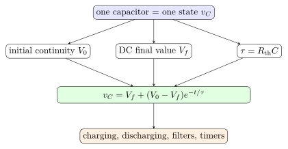
一阶 RC 的核心不是背诵两条特例,而是识别唯一状态变量 \(v_C\)。从拓扑分别得到 \(V_0\)、\(V_f\)、\(R_{\mathrm{th}}\),即可同时得到电压、电流、能量和时间尺度。滤波器则是同一动态方程在正弦稳态下的频域表现。
Formula-and-decision table / 公式与决策表
| Question | Relation | Conditions / limits |
|---|---|---|
| capacitor law | \(q=Cv_C\), \(i_C=C\,dv_C/dt\) | passive sign convention; constant \(C\) |
| voltage continuity | \(v_C(0^+)=v_C(0^-)\) | no ideal impulse current |
| general response | \(v_C=V_f+(V_0-V_f)e^{-t/\tau}\) | one independent capacitor; linear time-invariant resistive network after switching |
| time constant | \(\tau=R_{\mathrm{th}}C\) | resistance seen from capacitor port |
| initial slope | \(dv_C/dt\rvert_{0^+}=(V_f-V_0)/\tau\) | same first-order model |
| charging | \(v_C=\mathcal E(1-e^{-t/RC})\) | initially uncharged simple series RC |
| discharging | \(v_C=V_0e^{-t/RC}\) | zero Thevenin source after switching |
| low-pass | \(H=1/(1+\mathrm i\omega RC)\) | output across \(C\), sinusoidal steady state, unloaded |
| high-pass | \(H=\mathrm i\omega RC/(1+\mathrm i\omega RC)\) | output across \(R\), sinusoidal steady state, unloaded |
| cutoff | \(\omega_c=1/(RC)\), \(f_c=1/(2\pi RC)\) | ideal first-order filter |
| threshold time | \(t=-RC\ln(1-V_T/V_s)\) | zero initial voltage, \(0<V_T<V_s\) |
Model boundaries / 模型边界
- Lumped limit: circuit dimensions and propagation time must be small relative to signal wavelength and \(RC\).
- One-state limit: two independent capacitors generally produce two modes, not one \(\tau\).
- Linear components: dielectric absorption, voltage-dependent capacitance, temperature-dependent \(R\) and leakage can spoil a single exponential.
- Switch idealization: ideal switching can create discontinuous resistor current, but not finite capacitor-voltage jumps without an impulse.
- DC-final rule: capacitor-as-open applies only to constant-source steady state, not to AC or continuing transients.
- Filter loading: source resistance and load impedance alter gain and poles; the simple formulas assume ideal source and negligible loading.
- Frequency ceiling: parasitic inductance and ESR matter at sufficiently high frequency.
Misconception clinic / 误区诊所
- “电容在 \(t=0\) 一定是短路。” 只有初始电压为零时,\(0^+\) 的端口电压恰为零;一般应以保持 \(V_0\) 的电压源等效。
- “电容最终总是开路,所以一开始也能删掉。” 开路是直流终态结论,删除会丢失初始状态与暂态电流。
- “\(\tau\) 是充满所需时间。” 在一倍 \(\tau\) 时只完成 63.2%;严格达到终值需要无限时间。
- “时间常数就是图中任意一个 \(R\) 乘 \(C\)。” 应用的是电容端口所见 \(R_{\mathrm{th}}\)。
- “电流和电容电压同时上升。” 简单充电时 \(v_C\) 上升,而电流从最大值指数下降。
- “截止频率处输出为零。” 一阶滤波器在截止处幅度是通带值的 \(1/\sqrt2\),不是零。
- “磁场课程与本课无关。” 本课建立的 first-order state thinking 会在后续 RL、RLC 与场响应中继续出现,但元件的连续变量不同。
Practice and retrieval / 练习与提取
- [K01, 概念] 为什么有限电流不能使理想电容电压瞬间跳变?电流本身能否跳变?
- [K01, 定量] \(R=5.00\ \mathrm{k\Omega}\)、\(C=40.0\ \mathrm{\mu F}\)、\(\mathcal E=10.0\ \mathrm V\),初始未充电。求 \(t=0.200\ \mathrm s\) 的 \(v_C\) 和 \(i\)。
- [K01, 能量] \(100\ \mathrm{\mu F}\) 电容从 \(20.0\ \mathrm V\) 经电阻完全放电。电阻吸收多少能量?结果为何与 \(R\) 无关?
- [K02, 图像] 一条上升指数曲线的初始值 \(2.0\ \mathrm V\)、终值 \(8.0\ \mathrm V\),在 \(t=0\) 的切线于 \(0.50\ \mathrm s\) 处穿过终值线。写出函数。
- [K02, 估计] 响应进入终值的 \(\pm1.0\%\) 需要至少多少个时间常数?
- [K03, 网络] 电容从一个 \(15.0\ \mathrm V\) 初态接到 \(6.0\ \mathrm V\)、\(R_{\mathrm{th}}=3.00\ \mathrm{k\Omega}\) 的网络,\(C=10.0\ \mathrm{\mu F}\)。写出 \(v_C(t)\) 和 \(i_C(0^+)\)。
- [K03, 判断] 有受控源的网络求 \(R_{\mathrm{th}}\) 时,为什么不能把受控源关闭?应如何做?
- [K04, 滤波] \(R=10.0\ \mathrm{k\Omega}\)、\(C=15.9\ \mathrm{nF}\) 的低通截止频率是多少?在截止频率处幅度比和相位是多少?
- [K04, 高通] 对同一串联 RC,输出取在 \(R\) 上。说明 \(\omega\to0\) 与 \(\omega\to\infty\) 的极限,并给出物理解释。
- [综合, 定时] \(V_s=9.00\ \mathrm V\),\(C=22.0\ \mathrm{\mu F}\),希望从零充电到阈值 \(V_T=6.00\ \mathrm V\) 用 \(0.500\ \mathrm s\)。求所需 \(R\)。
Answers / 答案
1. \(\Delta v_C=C^{-1}\int i\,dt\);有限 \(i\) 乘零时间积分为零。理想开关可使电流有限跳变,因为电阻不储存状态。
2. \(\tau=0.200\ \mathrm s\),所以 \(v_C=10.0(1-e^{-1})=6.32\ \mathrm V\),\(i=(10.0/5000)e^{-1}=0.736\ \mathrm{mA}\)。
3. \(E=CV^2/2=0.0200\ \mathrm J\)。\(R\) 改变耗散速率与时间尺度,但时间积分等于初始场能。
4. \(\tau=0.50\ \mathrm s\),\(v_C(t)=8.0-6.0e^{-t/(0.50\ \mathrm s)}\ \mathrm V\)。
5. 要 \(e^{-t/\tau}\le0.010\),故 \(t/\tau\ge-\ln0.010=4.605\),至少约 \(4.61\tau\);工程上常取 \(5\tau\)。
6. \(\tau=(3000)(10.0\times10^{-6})=0.0300\ \mathrm s\),\(v_C=6.0+9.0e^{-t/(0.0300\ \mathrm s)}\ \mathrm V\);\(i_C(0^+)=(6.0-15.0)/3000=-3.00\ \mathrm{mA}\)。
7. 受控源由电路变量决定,关闭会改变端口物理。保留受控源,在端口施加测试电压或电流,取 \(R_{\mathrm{th}}=V_{test}/I_{test}\)。
8. \(f_c=[2\pi(10.0\times10^3)(15.9\times10^{-9})]^{-1}=1.00\ \mathrm{kHz}\);\(\lvert H\rvert=1/\sqrt2=0.707\),\(\phi=-45.0^\circ\)。
9. \(\omega\to0\) 时 \(Z_C\to\infty\)、电流和 \(V_R\) 趋零;\(\omega\to\infty\) 时 \(Z_C\to0\)、\(V_R\to V_{in}\)。
10. \(0.500=-RC\ln(1-6/9)=RC\ln3\),所以 \(R=0.500/[22.0\times10^{-6}\ln3]=20.7\ \mathrm{k\Omega}\)。
Exit ticket
- 不写“充电公式”,只用 \(V_0\)、\(V_f\)、\(R_{\mathrm{th}}\) 与 \(C\) 给出一阶 RC 的通用解和初始斜率。
- 说明同一个串联 RC 为什么既可做低通也可做高通,以及输出端选择如何改变物理意义。
Exit-ticket benchmark
\(v_C=V_f+(V_0-V_f)e^{-t/(R_{\mathrm{th}}C)}\),且 \(dv_C/dt\rvert_{0^+}=(V_f-V_0)/(R_{\mathrm{th}}C)\)。串联电流相同:低频主要压降在电容,高频主要压降在电阻;因此取电容电压得到低通,取电阻电压得到高通。
References and source notes / 参考资料与来源说明
Source-to-content map
| Source | Used for | Knowledge ID / section | Model boundary or convention |
|---|---|---|---|
| OpenStax University Physics Vol. 2, §10.5 RC Circuits | charging/discharging derivations, \(0.632/0.368\), timing applications | K01–K04 | ideal lumped \(R,C\) and DC source |
| MIT OCW 8.02T, RC Circuits presentation | KVL derivation, transient graphs, time constant | K01–K03 | passive sign convention normalized in this note |
| MIT OCW 8.02T, Experiment 04 | measurement of exponential response and nonideal laboratory context | K01–K03 | scope includes instrument and component uncertainty |
| MIT OCW 6.002, Lecture 18: Filters | low/high-pass transfer functions and frequency response | K04 | sinusoidal steady state, linear unloaded model |
| MIT OCW 2.003, First-Order System Notes | state/initial/final/time-constant interpretation | K02–K03 | general first-order linear-system analogy |
| NIST Special Publication 628 | RC integrator behavior in pulse-measurement practice | K04 | practical bandwidth and time-constant limitations |
资料和链接实际核对日期:2026-08-26。正文依据这些来源重新组织;全部图由本课方程原创绘制,未复制教材插图。
复习与拓展
- 在 AC circuits 中把 \(\mathrm i\omega\) 推广为 \(s\),区分 natural、forced 与 complete response。
- 在 RLC circuits 中比较电容电压连续性与电感电流连续性,并观察二阶过冲。
- 实验扩展:用示波器拟合 \(\ln\lvert v_C-V_f\rvert\) 对 \(t\) 的直线斜率。
- 工程扩展:加入 source resistance、load、ESR 与 leakage 后重新求 pole。