
Learning objectives / 学习目标
完成本课后,你应当能够:
- 定义 magnetization \(\mathbf M\),从其空间分布计算 \(\mathbf J_{\mathrm b}=\nabla\times\mathbf M\) 与 \(\mathbf K_{\mathrm b}=\mathbf M\times\hat{\mathbf n}\)。
- 由 \(\mathbf H=\mathbf B/\mu_0-\mathbf M\) 推导 \(\nabla\times\mathbf H=\mathbf J_{\mathrm f}\),并区分 \(\mathbf B,\mathbf H,\mathbf M\) 的单位与来源账本。
- 用磁化率、温度依赖和非线性/历史依赖区分 diamagnetic、paramagnetic、ferromagnetic response。
- 解释磁畴重排、饱和、剩磁、矫顽场和磁滞回线面积的能量意义。
- 推导并应用磁介质界面的 \(\mathbf B\) 法向与 \(\mathbf H\) 切向边界条件。
Prerequisites / 先修知识
- Forces and Torques on Currents:\(\boldsymbol\mu\)、力矩与偶极能。
- Biot–Savart Law:电流分布产生 \(\mathbf B\)。
- Ampère's Law:\(\nabla\times\mathbf B=\mu_0\mathbf J\)。
- curl、散度、pillbox 与 infinitesimal loop。
Scope and conventions / 范围与约定
- 采用经典连续介质宏观平均;平均尺度远大于原子尺度、远小于器件尺度。
- 总电流拆成 \(\mathbf J=\mathbf J_{\mathrm f}+\mathbf J_{\mathrm b}\);下标 f 表 free,b 表 bound。
- 材料表面外法向用于 \(\mathbf K_{\mathrm b}=\mathbf M\times\hat{\mathbf n}\)。
- 界面法向 \(\hat{\mathbf n}_{12}\) 从介质 1 指向介质 2;free surface current 为 \(\mathbf K_{\mathrm f}\)。
- SI 中 \(\mathbf B\) 单位 T,\(\mathbf H\) 与 \(\mathbf M\) 都是 \(\mathrm{A\,m^{-1}}\),但不是同一个场。
- 线性、各向同性、均匀关系 \(\mathbf M=\chi_m\mathbf H\) 只在指定材料与场强范围内使用;铁磁滞回通常不满足单值线性关系。
Notation and modeling contract / 符号与建模契约
| Symbol | Meaning | SI unit |
|---|---|---|
| \(\boldsymbol\mu\) | microscopic or localized magnetic dipole moment | \(\mathrm{A\,m^2}\) |
| \(\mathbf M=d\boldsymbol\mu/d\tau\) | magnetization, dipole moment per volume | \(\mathrm{A\,m^{-1}}\) |
| \(\mathbf J_{\mathrm b}\) | bound volume-current density | \(\mathrm{A\,m^{-2}}\) |
| \(\mathbf K_{\mathrm b}\) | bound surface-current density | \(\mathrm{A\,m^{-1}}\) |
| \(\mathbf H=\mathbf B/\mu_0-\mathbf M\) | auxiliary magnetic field | \(\mathrm{A\,m^{-1}}\) |
| \(\chi_m\) | magnetic susceptibility | dimensionless |
| \(\mu=\mu_0(1+\chi_m)\) | permeability in linear isotropic material | \(\mathrm{H\,m^{-1}}\) |
| \(\mathbf K_{\mathrm f}\) | free surface-current density at interface | \(\mathrm{A\,m^{-1}}\) |
Knowledge 1 — Magnetization and bound currents / 磁化与束缚电流
Knowledge ID: P04-U07-L03-K01
1.1 From dipoles to a continuum field
取足够小但含大量原子/分子的体积 \(\Delta\tau\),定义
\[\mathbf M(\mathbf r)=\lim_{\Delta\tau\to\mathrm{macro\ small}} \frac{\sum_{\Delta\tau}\boldsymbol\mu_i}{\Delta\tau}.\]
\(\mathbf M\) 是磁偶极矩密度,不是磁场。总体磁矩为
\[\boldsymbol\mu_{\mathrm{tot}}=\int_V\mathbf M\,d\tau.\]
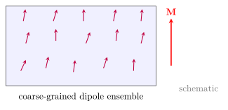
图 1 表示微观磁矩经空间平均形成 \(\mathbf M\);箭头并非单个磁针的真实尺寸。
1.2 Equivalent bound currents
磁化分布的外部与宏观内部场,可等效为
\[\boxed{\mathbf J_{\mathrm b}=\nabla\times\mathbf M}, \qquad \boxed{\mathbf K_{\mathrm b}=\mathbf M\times\hat{\mathbf n}}.\]
均匀 \(\mathbf M\) 的体内 curl 为零,但表面一般仍有束缚电流;“体内无 \(\mathbf J_{\mathrm b}\)”不等于“磁化不产生场”。
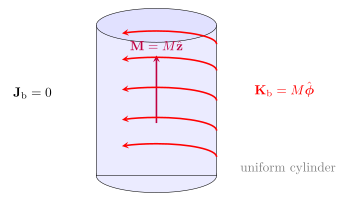
图 2 的均匀磁化圆柱等效于绕在表面的理想 sheet current;端面上 \(\mathbf M\times\hat{\mathbf n}=0\)。
1.3 Spatially varying magnetization
若 \(\mathbf M=M_y(x)\hat{\mathbf y}\),则
\[\mathbf J_{\mathrm b} =\nabla\times\mathbf M =\frac{dM_y}{dx}\hat{\mathbf z}.\]
因此 magnetization gradient 可产生体束缚电流,方向由 curl 而非由“磁矩箭头朝向”直接猜测。
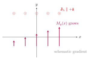
图 3 是 curl 的局部示意:向右增大的 \(M_y\) 对应 \(+z\) 束缚体电流。
Knowledge 2 — Auxiliary field \(\mathbf H\) / 辅助场 \(\mathbf H\)
Knowledge ID: P04-U07-L03-K02
2.1 Free-current bookkeeping
总场满足
\[\nabla\times\mathbf B =\mu_0(\mathbf J_{\mathrm f}+\mathbf J_{\mathrm b}) =\mu_0(\mathbf J_{\mathrm f}+\nabla\times\mathbf M).\]
定义
\[\boxed{\mathbf H\equiv\frac{\mathbf B}{\mu_0}-\mathbf M},\]
便有
\[\boxed{\nabla\times\mathbf H=\mathbf J_{\mathrm f}}, \qquad \boxed{\oint_C\mathbf H\cdot d\boldsymbol\ell=I_{\mathrm f,enc}}.\]
\(\mathbf H\) 是把材料束缚电流从 Ampère 账本中移走的 auxiliary field;它不是比 \(\mathbf B\) “更真实”或“更外加”的场。
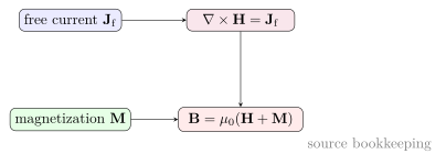
图 4 显示 \(\mathbf H\) 只让自由电流出现在 curl 方程右端;最终受力与磁通仍常用 \(\mathbf B\)。
2.2 Constitutive relation is extra physics
Maxwell equations 本身不给材料响应。在线性、各向同性、均匀且无明显历史依赖的范围内,可加
\[\mathbf M=\chi_m\mathbf H,\qquad \mathbf B=\mu_0(1+\chi_m)\mathbf H=\mu\mathbf H.\]
若材料各向异性,\(\chi_m\) 是 tensor;若铁磁响应非线性且有磁滞,\(\mathbf M\) 不是 \(\mathbf H\) 的单值线性函数。
Knowledge 3 — Diamagnetism, paramagnetism, and ferromagnetism / 抗磁、顺磁与铁磁
Knowledge ID: P04-U07-L03-K03
3.1 Response classes
- Diamagnetism(抗磁性): 外场诱导与外场反向的磁矩,\(\chi_m<0\);所有材料都有此量子起源响应,但常被更强机制掩盖。
- Paramagnetism(顺磁性): 已有微观磁矩在外场中略偏向排列,\(\chi_m>0\) 且通常很小;热涨落抵抗排列。
- Ferromagnetism(铁磁性): exchange interaction 支持协同有序,响应强、非线性且常有磁畴与历史依赖。
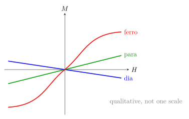
图 5 故意不按共同纵轴比例:顺/抗磁斜率通常远小于铁磁响应;颜色只区分类别。
3.2 Temperature and saturation
简单弱场顺磁模型常给 Curie law
\[\chi_m=\frac{C}{T},\]
更一般的铁磁高温相可近似 Curie–Weiss form \(\chi_m=C/(T-\Theta)\)。它们都有适用温区与弱场条件;低温或强场时量子能级和 saturation 使简单式失效。
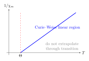
图 6 用 \(1/\chi_m\) 对 \(T\) 的线性化展示参数 \(\Theta\);相变附近不能盲目外推。
Knowledge 4 — Magnetic domains and hysteresis / 磁畴与磁滞
Knowledge ID: P04-U07-L03-K04
4.1 Domains reduce energy
铁磁体常分成多个 magnetic domains,各域内磁化接近饱和但方向不同,使宏观净磁矩降低。外场可驱动 domain-wall motion 与 moment rotation;缺陷会 pin 畴壁,使过程具有不可逆性。
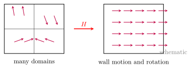
图 7 比较去磁宏观态与外场作用下的畴重排;不是把每个原子磁矩单独旋转成完全相同方向。
4.2 Hysteresis loop and energy loss
磁滞回线上关键量包括 saturation、remanence \(B_r\) 与 coercive field \(H_c\)。一个准静态循环的单位体积耗散能量等于回线面积的绝对值:
\[w_{\mathrm{loss}}=\left\lvert\oint H\,dB\right\rvert.\]
它的单位是 \((\mathrm{A\,m^{-1}})(\mathrm T)=\mathrm{J\,m^{-3}}\)。软磁材料通常窄回线、低损耗;永磁材料需要较大 coercivity,但真实选材还受温度、频率和机械加工影响。
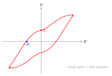
图 8 中路径有方向;回线面积是耗散,而不是任一时刻储存的全部磁能。
Knowledge 5 — Boundary conditions in magnetic media / 磁介质界面边界条件
Knowledge ID: P04-U07-L03-K05
5.1 Normal \(\mathbf B\) and tangential \(\mathbf H\)
令 \(\hat{\mathbf n}_{12}\) 从介质 1 指向介质 2。由 \(\nabla\cdot\mathbf B=0\) 的薄 pillbox:
\[\boxed{\hat{\mathbf n}_{12}\cdot(\mathbf B_2-\mathbf B_1)=0}.\]
由 \(\nabla\times\mathbf H=\mathbf J_{\mathrm f}\) 的薄矩形:
\[\boxed{\hat{\mathbf n}_{12}\times(\mathbf H_2-\mathbf H_1)=\mathbf K_{\mathrm f}}.\]
等价地,切向跳跃满足
\[\mathbf H_{2t}-\mathbf H_{1t} =\mathbf K_{\mathrm f}\times\hat{\mathbf n}_{12}.\]
若无自由面电流,\(\mathbf H_t\) 连续;无论材料如何,\(\mathbf B_n\) 连续。\(\mathbf B_t\) 与 \(\mathbf H_n\) 一般不连续。
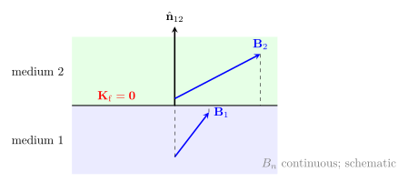
图 9 取界面为水平线、\(\hat{\mathbf n}_{12}\) 从 medium 1 指向 medium 2,并明确采用 \(\mathbf K_{\mathrm f}=\mathbf 0\)。因此两侧 \(\mathbf B\) 的法向分量相同、\(\mathbf H\) 的切向分量连续,而 \(\mathbf B\) 的切向分量可因 permeability 不同而改变;零面电流没有可画的方向箭头。
5.2 Refraction in linear media
若 \(\mathbf K_{\mathrm f}=0\) 且两侧线性各向同性,\(B_{1n}=B_{2n}\)、\(H_{1t}=H_{2t}\)。因 \(B_t=\mu H_t\),有
\[\frac{\tan\theta_2}{\tan\theta_1}=\frac{\mu_2}{\mu_1},\]
其中 \(\theta_i\) 从法线量起。该“折射”关系不是光的 Snell law,且在非线性、各向异性或有 surface current 时不能直接使用。
5.3 Boundary workflow
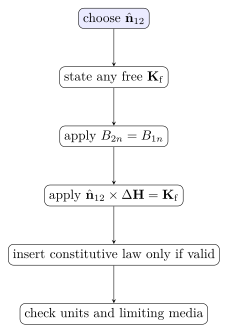
图 10 强调先用普遍边界条件,再加入材料关系;不能把 \(\mathbf B=\mu\mathbf H\) 当成所有介质的普遍定律。
Worked Examples / 完整例题
Worked Example 1 — Uniformly magnetized cylinder / 均匀磁化圆柱
已知: 圆柱 \(R=1.00\ \mathrm{cm}\)、\(L=5.00\ \mathrm{cm}\),\(\mathbf M=4.00\times10^5\hat{\mathbf z}\ \mathrm{A\,m^{-1}}\)。
对象与模型: 宏观均匀磁化、圆柱外为真空;侧面外法向 \(\hat{\mathbf r}\)。
\[\mathbf J_{\mathrm b}=\nabla\times\mathbf M=0,\qquad \mathbf K_{\mathrm b}=\mathbf M\times\hat{\mathbf r} =M\hat{\boldsymbol\phi}.\]
\[V=\pi R^2L=1.57\times10^{-5}\ \mathrm{m^3},\qquad \mu_{\mathrm{tot}}=MV=6.28\ \mathrm{A\,m^2}.\]
穿过一条母线的等效总环向电流为 \(K_{\mathrm b}L=2.00\times10^4\ \mathrm A\);与面积 \(\pi R^2\) 相乘仍给 \(6.28\ \mathrm{A\,m^2}\)。
检查: \(\mathbf K_{\mathrm b}\) 单位 A/m,乘长度才是 A;端面 \(\hat{\mathbf n}=\pm\hat{\mathbf z}\),故无表面束缚电流。
Worked Example 2 — Linear paramagnet in a solenoid / 线性顺磁体
已知: 长 solenoid 的 \(n=1500\ \mathrm{m^{-1}}\)、\(I=0.800\ \mathrm A\),填入 \(\chi_m=2.50\times10^{-4}\) 的线性顺磁体。
系统与模型: 忽略端部和退磁场,free current 决定 \(H=nI\)。
\[H=nI=1.20\times10^3\ \mathrm{A\,m^{-1}}, \qquad M=\chi_mH=0.300\ \mathrm{A\,m^{-1}}.\]
\[B=\mu_0(H+M) =(4\pi\times10^{-7})(1200.3) =1.51\times10^{-3}\ \mathrm T.\]
检查: \(\chi_m>0\) 使 \(B\) 略大于真空值;由于 \(\chi_m\) 很小,三位有效数字下增量不可见,但模型方向正确。
Worked Example 3 — Field refraction at an interface / 界面场折转
已知: \(\mu_1=2\mu_0\)、\(\mu_2=5\mu_0\),无 free surface current。介质 1 中 \(B_1=0.0200\ \mathrm T\),与法线夹角 \(\theta_1=30.0^\circ\)。
边界与坐标: \(\hat{\mathbf n}_{12}\) 从 1 指向 2,切向取 \(+x\)。两侧线性各向同性。
\[B_{2n}=B_{1n}=B_1\cos30^\circ=0.0173\ \mathrm T.\]
\[H_{2t}=H_{1t} \Rightarrow B_{2t}=\frac{\mu_2}{\mu_1}B_{1t} =\frac52(0.0200\sin30^\circ) =0.0250\ \mathrm T.\]
\[B_2=\sqrt{B_{2n}^2+B_{2t}^2}=0.0304\ \mathrm T, \qquad \theta_2=\tan^{-1}\frac{B_{2t}}{B_{2n}}=55.3^\circ.\]
检查: 法向分量相同;更大 \(\mu\) 使 \(\mathbf B\) 更趋向界面切向。三位有效数字。
Worked Example 4 — Hysteresis power loss / 磁滞功率损耗
已知: 某铁芯 \(B\)–\(H\) 回线面积为 \(1.80\times10^4\ \mathrm{J\,m^{-3}}\),体积 \(V=2.00\times10^{-5}\ \mathrm{m^3}\),循环频率 \(f=60.0\ \mathrm{Hz}\)。
系统与模型: 把铁芯作为热力学系统,准周期稳定循环;忽略涡流及其他损耗以隔离磁滞项。
\[E_{\mathrm{cycle}}=w_{\mathrm{loss}}V =(1.80\times10^4)(2.00\times10^{-5}) =0.360\ \mathrm J.\]
\[P=fE_{\mathrm{cycle}}=(60.0)(0.360)=21.6\ \mathrm W.\]
检查与解释: J/cycle 乘 cycles/s 得 W;真实铁芯总损耗还包括 eddy-current 与异常损耗。
Lesson synthesis / 本课综合
材料磁性问题有三张账本:\(\mathbf M\) 记录偶极矩密度并可转成 bound currents;\(\mathbf H\) 把 Ampère 环流右端整理成 free current;\(\mathbf B=\mu_0(\mathbf H+\mathbf M)\) 是最终总磁场。材料关系、磁畴动力学和磁滞是额外物理,不由 Maxwell 方程自动给出。界面上先用普遍的 \(B_n\) 与 \(H_t\) 跳跃条件,再使用合适 constitutive law。
Formula-and-decision table / 公式与决策表
| Task | Relation | Conditions / warning |
|---|---|---|
| Convert magnetization to sources | \(\mathbf J_{\mathrm b}=\nabla\times\mathbf M\), \(\mathbf K_{\mathrm b}=\mathbf M\times\hat{\mathbf n}\) | material outer normal for \(\mathbf K_{\mathrm b}\) |
| Separate free current | \(\mathbf H=\mathbf B/\mu_0-\mathbf M\) | definition in macroscopic SI |
| Ampère law for free current | \(\nabla\times\mathbf H=\mathbf J_{\mathrm f}\) | magnetostatics |
| Linear material | \(\mathbf M=\chi_m\mathbf H\), \(\mathbf B=\mu\mathbf H\) | linear, isotropic, stated range |
| Hysteresis loss | \(w_{\mathrm{loss}}=\lvert\oint H\,dB\rvert\) | full stabilized cycle |
| Any interface | \(B_{2n}=B_{1n}\) | no magnetic monopoles |
| Interface with free sheet current | \(\hat{\mathbf n}_{12}\times(\mathbf H_2-\mathbf H_1)=\mathbf K_{\mathrm f}\) | orientation must be declared |
Model boundaries / 模型边界
- 连续 \(\mathbf M\) 是宏观平均,不描述单个 spin 或晶格尺度结构。
- \(\mathbf M=\chi_m\mathbf H\) 不适用于饱和、磁滞、强非线性、明显各向异性或频率色散。
- Curie/Curie–Weiss laws 有温区和弱场限制,不能穿过相变点机械外推。
- 理想回线面积公式假设稳定周期;动态磁滞会随频率和波形改变。
- 界面折转式要求线性各向同性且 \(\mathbf K_{\mathrm f}=0\);普遍边界条件本身不要求这些。
- 微观磁性根源涉及量子力学;本课只建立本科宏观场论接口。
Misconception clinic / 误区诊所
- 把 \(\mathbf M\) 当作 T。 它是磁矩密度,单位 A/m。
- 均匀 \(\mathbf M\) 所以没有 bound current。 只有体束缚电流为零,表面 \(\mathbf K_{\mathrm b}\) 可非零。
- \(\mathbf H\) 只由外加场产生。 它是由 \(\mathbf B\) 与 \(\mathbf M\) 定义的辅助场,不等同于“外场”。
- \(\mu_r\) 是材料永恒常数。 非线性、温度、频率、方向和历史都可使其变化。
- 铁磁体零外场时每个磁矩随机。 域内高度有序;去磁态是不同磁畴宏观抵消。
- 界面上 \(\mathbf B\) 全矢量连续。 只有法向分量普遍连续;切向分量可跳变。
- 回线面积是瞬时储能。 它是一周期耗散能量密度。
Practice and retrieval / 练习与提取
- 定义(K01): 均匀 \(\mathbf M=M\hat{\mathbf z}\) 的长圆柱有哪些 bound currents?
- curl(K01): 若 \(\mathbf M=kx\,\hat{\mathbf y}\),求 \(\mathbf J_{\mathrm b}\)。
- H field(K02): 某点 \(\mathbf B=0.020\hat{\mathbf x}\ \mathrm T\)、\(\mathbf M=5.0\times10^3\hat{\mathbf x}\ \mathrm{A\,m^{-1}}\),求 \(\mathbf H\)。
- 线性介质(K02): \(\chi_m=-1.0\times10^{-5}\)、\(H=2.0\times10^4\ \mathrm{A\,m^{-1}}\),求 \(M\) 与 \(B\)。
- 分类(K03): 仅由 \(\chi_m>0\) 能否断言材料是 ferromagnet?解释。
- 温度(K03): 简单 Curie paramagnet 从 \(300\ \mathrm K\) 升至 \(600\ \mathrm K\),弱场 \(\chi_m\) 如何变化?
- 磁畴(K04): 为什么未磁化铁磁体仍可在每个 domain 内有大磁化?
- 磁滞(K04): 回线面积 \(5.0\times10^3\ \mathrm{J\,m^{-3}}\)、体积 \(1.0\times10^{-4}\ \mathrm{m^3}\)、频率 \(50\ \mathrm{Hz}\),求磁滞功率。
- 边界(K05): 无 free sheet current 时,哪些分量连续?
- 界面电流(K05): \(\hat{\mathbf n}_{12}=\hat{\mathbf z}\)、\(\mathbf K_{\mathrm f}=K\hat{\mathbf x}\),求 \(\mathbf H_{2t}-\mathbf H_{1t}\) 的方向与大小。
Answer
均匀 \(\mathbf M\) 给出 \(\mathbf J_{\mathrm b}=\nabla\times\mathbf M=0\);侧面 \(\mathbf K_{\mathrm b}=\mathbf M\times\hat{\mathbf n}=M\hat{\boldsymbol\phi}\),端面为零。
Answer
\(\nabla\times(kx\hat{\mathbf y})=k\hat{\mathbf z}\);若 \(k\) 的单位为 \(\mathrm{A\,m^{-2}}\),则 \(\mathbf J_{\mathrm b}\) 也为 \(\mathrm{A\,m^{-2}}\)。
Answer
\(\mathbf H=\mathbf B/\mu_0-\mathbf M=[0.020/(4\pi\times10^{-7})-5000]\hat{\mathbf x}=1.09\times10^4\hat{\mathbf x}\ \mathrm{A\,m^{-1}}\)。
Answer
\(M=\chi_mH=-0.200\ \mathrm{A\,m^{-1}}\);\(B=\mu_0(H+M)=2.51\times10^{-2}\ \mathrm T\)(三位有效数字)。
Answer
不能;paramagnet 也有小的正 \(\chi_m\)。还需检查响应强度、非线性、磁畴、剩磁和历史依赖。
Answer
在弱场 Curie 区间 \(\chi_m=C/T\),温度从 \(300\ \mathrm K\) 加倍到 \(600\ \mathrm K\) 时,\(\chi_m\) 减半。
Answer
exchange interaction 使每个磁畴内部有序;不同磁畴取向相消,仍可使宏观净磁矩接近零。
Answer
每周期耗散 \(E=(5.0\times10^3\ \mathrm{J\,m^{-3}})(1.0\times10^{-4}\ \mathrm{m^3})=0.50\ \mathrm J\);功率 \(P=Ef=(0.50\ \mathrm J)(50\ \mathrm{s^{-1}})=25\ \mathrm W\)。
Answer
无自由面电流时,\(B_n\) 与 \(H_t\) 连续;\(B_t\)、\(H_n\) 不必连续。
Answer
\(\Delta\mathbf H_t=\mathbf K_{\mathrm f}\times\hat{\mathbf n}_{12}=K\hat{\mathbf x}\times\hat{\mathbf z}=-K\hat{\mathbf y}\),大小为 \(K\),单位为 \(\mathrm{A\,m^{-1}}\)。
Exit ticket / 离堂检核
- 一块均匀磁化材料内部 \(\nabla\times\mathbf M=0\)。解释为何它仍可在外部产生磁场,并写出相应源。
- 有人说“界面无自由电流,所以 \(\mathbf B\) 连续”。指出错误,并给出正确的两条分量条件。
References and source notes / 参考资料与来源说明
Source-to-content map
| Source | Used for | Knowledge ID / section | Model boundary or convention |
|---|---|---|---|
| OpenStax University Physics Vol. 2, §12.7 Magnetism in Matter | dia/para/ferromagnetism, temperature, domains, hysteresis | K03, K04 | introductory macroscopic classification |
| UT Austin, Magnetization, Bound Currents, and the H Field | \(\mathbf J_{\mathrm b}\), \(\mathbf K_{\mathrm b}\), \(\mathbf H\), boundary conditions | K01, K02, K05 | SI definitions and interface orientation |
| MIT OCW 8.02, Chapter 9: Sources of Magnetic Fields | magnetic dipoles and material response | K01–K04 | independent undergraduate treatment |
| MIT OCW 8.02, Week 7 Presentation: Magnetic Materials | qualitative response classes and dipoles | K03, K04 | lecture-level conceptual cross-check |
| The Feynman Lectures on Physics, Vol. II, Ch. 34 | microscopic origins and magnetism of matter | K03 | classical/quantum boundary noted |
| The Feynman Lectures on Physics, Vol. II, Ch. 35: Paramagnetism and Magnetic Resonance | paramagnetism and thermal alignment | K03 | weak-field and temperature-dependent response |
| The Feynman Lectures on Physics, Vol. II, Ch. 36: Ferromagnetism | magnetization currents, \(\mathbf H\), domains, and ferromagnetism | K01–K04 | macroscopic/classical averaging and cooperative response |
| NIST Magnetic Moment and Susceptibility Standard Reference Material | susceptibility measurement and metrology context | K03 | real materials require calibrated measurements |
资料与链接实际浏览、阅读和核对日期:2026-08-28。不同来源的 \(\mathbf H\) 和界面法向约定已统一为本课声明;图示均为原创。
复习与拓展
- Faraday’s and Lenz’s Laws:时变 \(\mathbf B\) 与磁性材料中的感应。
- Magnetic circuits:在受控近似下用 reluctance,但不能忽略 fringing 与非线性。
- Thermodynamics of magnetic media:能量、功与选择 \(\mathbf B\) 或 \(\mathbf H\) 作为控制变量。
- Condensed matter:exchange、spin waves、anisotropy 与相变。