
Learning objectives / 学习目标
完成本课后,你应当能够:
- 以源点 \(\mathbf r'\)、场点 \(\mathbf r\) 和分离矢量 \(\mathbf R=\mathbf r-\mathbf r'\) 正确写出 Biot–Savart law,并用叉积判断方向。
- 从电流元积分推导有限直导线、圆弧和圆环轴线上的磁场。
- 对线电流、面电流和体电流选择正确积分元,进行矢量叠加并利用对称性消去分量。
- 定义电流环的磁偶极矩,推导其远场并估计偶极近似误差。
- 对结果执行量纲、方向、极限、连续性和数量级检查。
Prerequisites / 先修知识
- Electric Current and Conduction:\(I\)、\(\mathbf J\) 与稳恒电流。
- Magnetic Field and Lorentz Force:\(\mathbf B\) 的操作定义与右手定则。
- Forces and Torques on Currents:磁偶极矩的方向。
- 叉积、向量分量、单变量积分与多重积分。
Scope and conventions / 范围与约定
- 本课限于 magnetostatics(磁静力学):电流分布与电荷密度在所选惯性系中不随时间变化,并满足 \(\nabla\cdot\mathbf J=0\)。
- conventional current 的方向定义 \(d\boldsymbol\ell'\);电子漂移方向通常相反。
- 源点用撇号 \(\mathbf r'\),场点用 \(\mathbf r\);\(\mathbf R=\mathbf r-\mathbf r'\) 永远从源点指向场点。
- 采用 SI。真空磁导率 \(\mu_0\) 在 2019 SI 后是实验确定量;本课数值计算取 \(\mu_0\simeq4\pi\times10^{-7}\ \mathrm{N\,A^{-2}}\)。
- 理想细导线在自身中心线处的场会发散;实际导线必须用有限截面电流密度建模。
- 所有几何图均为 schematic / not to scale,除非另有说明。
Notation and modeling contract / 符号与建模契约
| Symbol | Meaning | SI unit |
|---|---|---|
| \(\mathbf r',\mathbf r\) | source point, field point | m |
| \(\mathbf R=\mathbf r-\mathbf r'\) | source-to-field displacement | m |
| \(R=\lvert\mathbf R\rvert\) | source-to-field distance | m |
| \(I\,d\boldsymbol\ell'\) | directed line-current element | \(\mathrm{A\,m}\) |
| \(\mathbf K,\mathbf J\) | surface and volume current density | \(\mathrm{A\,m^{-1}}\), \(\mathrm{A\,m^{-2}}\) |
| \(\mathbf B\) | magnetic flux density | T |
| \(\boldsymbol\mu=IA\hat{\mathbf n}\) | magnetic dipole moment of one loop | \(\mathrm{A\,m^2}\) |
| \(a,R_0\) | perpendicular distance; loop radius | m |
Knowledge 1 — Field of a current element / 电流元的磁场
Knowledge ID: P04-U07-L01-K01
1.1 Vector law and physical picture
对位于 \(\mathbf r'\) 的定向线元 \(d\boldsymbol\ell'\),稳恒电流 \(I\) 对场点 \(\mathbf r\) 的贡献为
\[d\mathbf B(\mathbf r) =\frac{\mu_0}{4\pi} \frac{I\,d\boldsymbol\ell'\times\mathbf R}{R^3}, \qquad \mathbf R=\mathbf r-\mathbf r'.\]
其大小是
\[dB=\frac{\mu_0}{4\pi}\frac{I\,d\ell'\sin\alpha}{R^2},\]
其中 \(\alpha\) 是 \(d\boldsymbol\ell'\) 与 \(\mathbf R\) 的夹角。于是有三个即时判断:贡献与 \(I\) 成正比、随距离平方衰减、与电流元平行的观察方向贡献为零。方向由 \(d\boldsymbol\ell'\times\mathbf R\) 的右手定则确定。
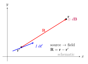
图 1 把三个方向分开:先画源到场的 \(\mathbf R\),再做叉积;不能把 \(\mathbf r\) 或 \(\mathbf r'\) 误当作分离矢量。
1.2 Angular factor and limits
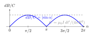
图 2 强调 \(\sin\alpha\) 不是装饰因子:轴向观察为零,垂直观察最大。若式子在 \(\alpha=0\) 仍给非零场,几何或叉积必有错误。
1.3 Complete-current integral
对完整的稳恒电流回路积分:
\[\mathbf B(\mathbf r)=\frac{\mu_0 I}{4\pi} \int_C\frac{d\boldsymbol\ell'\times(\mathbf r-\mathbf r')} {\lvert\mathbf r-\mathbf r'\rvert^3}.\]
量纲为 \((\mathrm{N\,A^{-2}})(\mathrm A)(\mathrm m)/(\mathrm{m^2})=\mathrm T\)。
Knowledge 2 — Straight wires, loops, and arcs / 直导线、圆环与圆弧
Knowledge ID: P04-U07-L01-K02
2.1 Finite straight wire
场点到直导线的垂距为 \(a\),两端相对垂足张角为 \(\theta_1,\theta_2\)(从垂线量起)。取导线沿 \(x\),则 \(R^2=a^2+x^2\),积分给
\[B=\frac{\mu_0 I}{4\pi} \int_{x_1}^{x_2}\frac{a\,dx}{(a^2+x^2)^{3/2}} =\frac{\mu_0 I}{4\pi a} (\sin\theta_1+\sin\theta_2).\]
无限长极限 \(\theta_1,\theta_2\to\pi/2\) 给 \(B=\mu_0I/(2\pi a)\)。
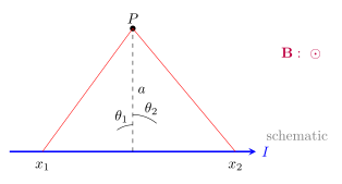
图 3 中电流向右、场点在上方,磁场出纸面。若 \(\theta_i\) 改从导线方向量起,公式中的三角函数也必须改变。
2.2 Circular arc and radial leads
半径 \(R_0\)、圆心角 \(\phi\)(弧度)的圆弧在圆心处有
\[B_{\mathrm{arc}}=\frac{\mu_0 I}{4\pi R_0}\int d\phi =\frac{\mu_0 I\phi}{4\pi R_0}.\]
若连接导线沿圆心径向延伸,则 \(d\boldsymbol\ell'\parallel\mathbf R\),其圆心场严格为零。
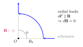
图 4 说明“导线存在”不等于“必有贡献”;必须检查叉积几何。
2.3 Field on the axis of a circular loop
环上相对线元的横向分量相消,轴向分量相加:
\[B_z(z)=\frac{\mu_0IR_0^2}{2(R_0^2+z^2)^{3/2}}.\]
在中心 \(B_z(0)=\mu_0I/(2R_0)\);当 \(z\gg R_0\),它按 \(z^{-3}\) 衰减。
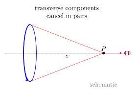
图 5 的每个 \(d\mathbf B\) 并非都沿轴;只有配对后横向分量才抵消。
Knowledge 3 — Superposition for current distributions / 电流分布的叠加
Knowledge ID: P04-U07-L01-K03
3.1 Vector superposition
真空磁静态方程对源线性:
\[\mathbf B_{\mathrm{net}}(\mathbf r)=\sum_i\mathbf B_i(\mathbf r).\]
必须先统一坐标再相加分量,不能直接相加磁场大小。
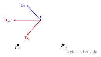
图 6 用矢量合成提示:不共线的两场必须保留方向。
3.2 Line, surface, and volume currents
\[\mathbf B(\mathbf r)=\frac{\mu_0}{4\pi} \int_C\frac{I\,d\boldsymbol\ell'\times\mathbf R}{R^3},\]
\[\mathbf B(\mathbf r)=\frac{\mu_0}{4\pi} \int_S\frac{\mathbf K(\mathbf r')\times\mathbf R}{R^3}\,da',\]
\[\mathbf B(\mathbf r)=\frac{\mu_0}{4\pi} \int_V\frac{\mathbf J(\mathbf r')\times\mathbf R}{R^3}\,d\tau'.\]
\(\mathbf K\) 单位为 \(\mathrm{A\,m^{-1}}\),\(\mathbf J\) 单位为 \(\mathrm{A\,m^{-2}}\);穿过截面 \(S\) 的电流是 \(I=\int_S\mathbf J\cdot d\mathbf a\)。
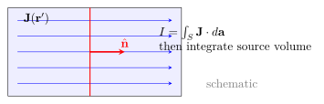
图 7 区分“由 \(\mathbf J\) 算穿面电流”和“对整个源体积算磁场”这两种不同积分。
3.3 Reliable symmetry workflow
- 声明源分布、场点和坐标系。
- 配对对称源元,先判断相消分量。
- 对保留分量积分,而不是先积分大小再猜方向。
- 用 \(I\to0\)、中心、远场或无限长极限检查。
Knowledge 4 — Far field of a current loop / 电流环的远场
Knowledge ID: P04-U07-L01-K04
4.1 Magnetic dipole moment
对面积 \(A\)、单位法向 \(\hat{\mathbf n}\) 的平面小回路,
\[\boldsymbol\mu=IA\hat{\mathbf n}.\]
当 \(r\) 远大于回路尺度 \(R_0\),
\[\mathbf B(\mathbf r)\simeq \frac{\mu_0}{4\pi r^3} \left[3(\boldsymbol\mu\cdot\hat{\mathbf r})\hat{\mathbf r}-\boldsymbol\mu\right].\]
轴线上 \(B_{\mathrm{axis}}=\mu_0\mu/(2\pi r^3)\);赤道面上 \(B_{\mathrm{eq}}=\mu_0\mu/(4\pi r^3)\),方向与 \(\boldsymbol\mu\) 相反。
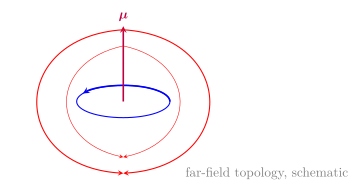
图 8 只表达远场拓扑。没有磁单极的 \(r^{-2}\) 项,这与 \(\nabla\cdot\mathbf B=0\) 一致。
4.2 Axial expansion and error
由圆环轴线精确式,令 \(u=R_0^2/z^2\):
\[B_z=\frac{\mu_0IR_0^2}{2z^3}(1+u)^{-3/2} =\frac{\mu_0\mu}{2\pi z^3} \left(1-\frac32u+O(u^2)\right).\]
偶极近似的相对首阶修正约 \(3R_0^2/(2z^2)\),所以“很远”应由 \(R_0/z\) 量化。
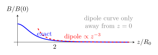
图 9 比较精确场与渐近式;偶极式在 \(z=0\) 发散,不能外推到回路中心。
4.3 Modeling decision
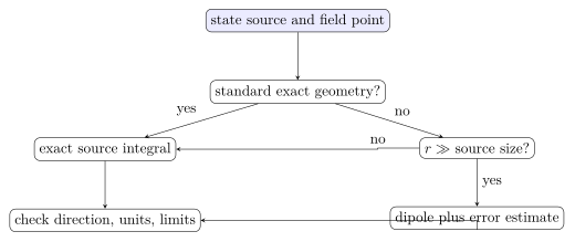
图 10 把选模型放在代数之前;exact 与 far-field approximation 不能混用。
Worked Examples / 完整例题
Worked Example 1 — Finite straight wire / 有限直导线
已知: \(I=4.00\ \mathrm A\),\(a=3.00\ \mathrm{cm}\),\(\theta_1=30.0^\circ\)、\(\theta_2=60.0^\circ\)。电流向右,场点在上方。
对象、参考系与模型: 导线与场点静止于实验室惯性系;细直导线、稳恒电流。\(+z\) 指出纸面。
\[B=\frac{\mu_0I}{4\pi a}(\sin\theta_1+\sin\theta_2) =\frac{10^{-7}(4.00)}{0.0300}(0.500+0.866) =1.82\times10^{-5}\ \mathrm T.\]
\[\boxed{\mathbf B=1.82\times10^{-5}\ \mathrm T\,\hat{\mathbf z}}.\]
检查: 小于同距无限长导线的 \(2.67\times10^{-5}\ \mathrm T\);单位、方向和三位有效数字均合理。
Worked Example 2 — Three-quarter arc / 四分之三圆弧
已知: \(I=2.50\ \mathrm A\),\(R_0=8.00\ \mathrm{cm}\),\(\phi=3\pi/2\),电流逆时针;两条引线沿径向。
对象与模型: 圆心为场点,纸外为 \(+z\);稳恒细导线。径向段叉积为零。
\[B=10^{-7}\frac{(2.50)(3\pi/2)}{0.0800} =1.47\times10^{-5}\ \mathrm T.\]
\[\boxed{\mathbf B=1.47\times10^{-5}\ \mathrm T\,\hat{\mathbf z}}.\]
检查: 它是同半径满圆场 \(1.96\times10^{-5}\ \mathrm T\) 的 \(0.750\) 倍,方向与比例均合理。
Worked Example 3 — Field on a loop axis / 圆环轴线场
已知: \(R_0=0.100\ \mathrm m\),\(I=3.00\ \mathrm A\),\(z=0.120\ \mathrm m\);从 \(+z\) 看电流逆时针。
对象与坐标: 圆环中心为原点,轴为 \(z\);稳恒细线圆环。
\[B_z=\frac{(4\pi\times10^{-7})(3.00)(0.100)^2} {2[(0.100)^2+(0.120)^2]^{3/2}} =4.95\times10^{-6}\ \mathrm T.\]
\[\boxed{\mathbf B=4.95\ \mathrm{\mu T}\,\hat{\mathbf z}}.\]
检查: 小于中心场 \(18.8\ \mathrm{\mu T}\),且分母三次方给出 T 量纲。
Worked Example 4 — Dipole approximation / 偶极近似
已知: \(I=1.20\ \mathrm A\)、\(R_0=0.0500\ \mathrm m\)、轴上 \(z=1.00\ \mathrm m\)。
模型理由: \(R_0/z=0.0500\ll1\),可用磁偶极项,再用精确式核验。
\[\mu=I\pi R_0^2=9.42\times10^{-3}\ \mathrm{A\,m^2}, \qquad B_{\mathrm{dip}}=\frac{\mu_0\mu}{2\pi z^3} =1.88496\ \mathrm{nT}.\]
精确式给 \(B_{\mathrm{exact}}=1.87791\ \mathrm{nT}\),相对高估
\[\frac{B_{\mathrm{dip}}-B_{\mathrm{exact}}}{B_{\mathrm{exact}}}=0.375\%.\]
检查: 首阶估计 \(3R_0^2/(2z^2)=0.375\%\) 与精确比较一致;结果方向沿 \(\boldsymbol\mu\)。
Lesson synthesis / 本课综合
Biot–Savart 建模依次处理:源—场几何、正确源测度、矢量对称配对、积分与尺度近似。近场保留几何细节;远离局域闭合电流时,首项由 \(\boldsymbol\mu\) 控制。每次都用方向、量纲、极限和无量纲近似参数复核。
Formula-and-decision table / 公式与决策表
| Situation | Use | Conditions and diagnostic |
|---|---|---|
| General thin steady wire | \(\mathbf B=\dfrac{\mu_0I}{4\pi}\int d\boldsymbol\ell'\times\mathbf R/R^3\) | full vector geometry; not on ideal wire |
| Finite straight wire | \(B=\dfrac{\mu_0I}{4\pi a}(\sin\theta_1+\sin\theta_2)\) | angles measured from perpendicular |
| Arc at center | \(B=\dfrac{\mu_0I\phi}{4\pi R_0}\) | \(\phi\) in radians; radial leads give zero |
| Circular-loop axis | \(B_z=\dfrac{\mu_0IR_0^2}{2(R_0^2+z^2)^{3/2}}\) | point is on axis |
| Surface or volume current | replace source by \(\mathbf K\,da'\) or \(\mathbf J\,d\tau'\) | vector integration |
| Far from localized loop | dipole field, \(\boldsymbol\mu=IA\hat{\mathbf n}\) | source size divided by \(r\) is small |
Model boundaries / 模型边界
- Steady source: 时间依赖电荷/电流或传播时延重要时,磁静态公式不完整。
- Thin wire: 在线半径尺度内必须用实际 \(\mathbf J\);理想线源自场奇异。
- Material background: 介质中的总场可由自由与束缚电流共同产生,Unit 4.7.3 将引入 \(\mathbf M,\mathbf H\)。
- Dipole approximation: 要求源尺度与 \(r\) 之比远小于 1;近场与回路中心禁用。
- Classical continuum: 原子尺度的离散电荷与量子磁矩需要更精细模型。
Misconception clinic / 误区诊所
- 把 \(\mathbf R\) 画成原点到场点。 它必须从每个源点指向场点。
- 积分 \(dB\) 大小后再猜方向。 方向随源点变时必须先投影或配对。
- 认为径向引线也贡献圆心场。 此时叉积为零。
- 角度定义改变却不改公式。 直线公式中的角必须从垂线量起。
- 认为任何电流场都按 \(1/r\) 衰减。 局域闭合环远场按 \(1/r^3\)。
- 把 \(\mu_0=4\pi\times10^{-7}\) 当作现行 SI 精确定义。 2019 SI 后它是测量量,课堂近似仍足够准确。
Practice and retrieval / 练习与提取
- 方向(K01): 电流元沿 \(+x\),场点相对源点在 \(+y\)。\(d\mathbf B\) 指向哪里?若场点在 \(-x\) 呢?
- 量纲(K01): 验证 Biot–Savart 微元式的 SI 单位为 T。
- 有限线(K02): \(I=6.0\ \mathrm A\),\(a=4.0\ \mathrm{cm}\),\(\theta_1=45^\circ\)、\(\theta_2=30^\circ\),求 \(B\)。
- 极限(K02): 从有限直导线式恢复半无限长导线场。
- 圆弧(K02): 半径 \(0.12\ \mathrm m\)、电流 \(3.0\ \mathrm A\) 的 \(120^\circ\) 圆弧在圆心产生多大磁场?
- 函数(K02): 求圆环轴线上 \(\lvert dB_z/dz\rvert\) 最大的位置,并检验“最大处为 \(z=R_0/\sqrt2\)”这一说法。
- 叠加(K03): 两无限长平行导线相距 \(0.20\ \mathrm m\),均载流 \(5.0\ \mathrm A\)。中点场在同向和反向时各是多少?
- 源模型(K03): 写出均匀 \(\mathbf J=J_0\hat{\mathbf z}\) 中小体积元的 \(d\mathbf B\)。
- 远场(K04): \(I=2.0\ \mathrm A\)、\(R_0=3.0\ \mathrm{cm}\) 的圆环磁矩是多少?轴线 \(r=0.50\ \mathrm m\) 处偶极场是多少?
- 边界(K04): \(R_0/r=0.20\) 时,估计轴上偶极近似相对误差。能否满足 \(1\%\) 精度?
Answer
\(\hat{\mathbf x}\times\hat{\mathbf y}=\hat{\mathbf z}\),故为 \(+z\);在 \(-x\) 时两矢量平行或反平行,场为零。
Answer
\((\mathrm{N\,A^{-2}})(\mathrm A)(\mathrm m)/\mathrm{m^2}=\mathrm{N/(A\,m)}=\mathrm T\)。
Answer
\(B=10^{-7}(6.0/0.040)(\sin45^\circ+\sin30^\circ)=1.81\times10^{-5}\ \mathrm T\)。
Answer
取一端 \(\theta=90^\circ\)、另一端 \(\theta=0\),得 \(B=\mu_0I/(4\pi a)\)。
Answer
\(\phi=2\pi/3\),\(B=\mu_0I\phi/(4\pi R_0)=5.24\times10^{-6}\ \mathrm T\)。
Answer
\(\lvert dB_z/dz\rvert\) 是偶函数;在 \(z>0\),它正比于 \(z(R_0^2+z^2)^{-5/2}\)。求导得 \(R_0^2-4z^2=0\),所以整条轴线上的两个最大处为 \(\lvert z\rvert=R_0/2\)。题目中的 \(R_0/\sqrt2\) 说法不成立,这正是函数检查要发现的错误。
Answer
同向时中点两场反向,净场 0;反向时相加,每根 \(1.00\times10^{-5}\ \mathrm T\),净场 \(2.00\times10^{-5}\ \mathrm T\)。
Answer
\(d\mathbf B=\dfrac{\mu_0}{4\pi}\dfrac{J_0\hat{\mathbf z}\times(\mathbf r-\mathbf r')}{\lvert\mathbf r-\mathbf r'\rvert^3}\,d\tau'\)。
Answer
\(\mu=I\pi R_0^2=5.65\times10^{-3}\ \mathrm{A\,m^2}\);\(B\simeq\mu_0\mu/(2\pi r^3)=9.05\times10^{-9}\ \mathrm T\)。
Answer
首阶修正约 \((3/2)(0.20)^2=6.0\%\),不满足 \(1\%\),应使用精确式。
Exit ticket / 离堂检核
- 不积分,解释圆环轴线场为什么只能沿轴;再说明为何对称性不能独自确定幅值。
- 一位同学在距圆环中心两倍半径处使用偶极式。给出无量纲误差估计并提出更可靠方法。
References and source notes / 参考资料与来源说明
Source-to-content map
| Source | Used for | Knowledge ID / section | Model boundary or convention |
|---|---|---|---|
| OpenStax University Physics Vol. 2, §12.1 The Biot–Savart Law | vector law, current-element geometry, superposition | K01, K03 | steady currents; SI vector convention |
| OpenStax University Physics Vol. 2, §12.2 Magnetic Field Due to a Thin Straight Wire | finite and infinite straight-wire derivation | K02 | thin-wire idealization |
| OpenStax University Physics Vol. 2, §12.4 Magnetic Field of a Current Loop | arcs, loop-axis field, loop far field | K02, K04 | exact axis result and far limit |
| MIT OCW 8.02, Chapter 9: Sources of Magnetic Fields | independent derivations and dipole comparison | K01–K04 | magnetostatic source model |
| The Feynman Lectures on Physics, Vol. II, Ch. 14 | fields of wires and coils; physical interpretation | K02–K04 | classical field description |
| NIST CODATA 2022 recommended values | value and uncertainty of \(\mu_0\) | Scope | post-2019 SI: measured, not exact |
| BIPM SI Brochure Appendix 2: Practical realization of the ampere | SI-redefinition context | Scope, misconceptions | exact elementary charge defines ampere |
资料与链接实际浏览、阅读和核对日期:2026-08-28。正文为重新组织的教学表述;全部图示依据方程原创绘制,未复制来源插图。
复习与拓展
- Ampère's Law:在高度对称源中,用环流快速得到同一磁场。
- Magnetism in Matter:把原子磁矩集合描述为 \(\mathbf M\) 与束缚电流。
- Boundary-Value and Multipole Methods:系统化电、磁多极展开。
- Electrodynamics:时间依赖源、retarded potentials 与辐射。