
Learning objectives / 学习目标
完成本课后,你应能:
- 区分 temporal coherence 与 spatial coherence,并指出它们分别比较同一场在不同时刻和不同位置的相关性。
- 在明确谱线形状和阈值定义后计算 coherence time 与 coherence length,并解释为何不存在唯一通用因子。
- 使用 mutual coherence function 推导一般双束强度与 visibility,分离强度失配和失相干。
- 画出 Michelson、Mach–Zehnder、Sagnac 的真实光路,正确识别单程/双程、公共路径和敏感物理量。
- 由条纹数或相位分数求位移、折射率与旋转相位,并建立包含波长、环境、几何、相位拟合的误差账本。
Prerequisites / 先修知识
- 双束相位与 visibility。
- 多束干涉与腔线宽。
- 波包、谱宽和群延迟。
- 复数共轭、时间平均、Fourier transform 的基本概念和不确定度传播。
Scope and conventions / 范围与约定
- 使用解析信号或准单色复场 \(E(\mathbf r,t)\);角括号 \(\langle\cdot\rangle\) 表示比光学周期长、比实验漂移短的系综或时间平均。
- mutual coherence 的共轭放在第一个场:
\[\Gamma_{12}(\tau) =\left\langle E_1^*(t)E_2(t+\tau)\right\rangle.\]
- normalized degree of coherence 为
\[\gamma_{12}(\tau) =\frac{\Gamma_{12}(\tau)} {\sqrt{\Gamma_{11}(0)\Gamma_{22}(0)}}.\]
- 真空中的延迟与 OPD 关系为 \(\tau=\Delta/c\)。色散介质的包络延迟使用 group index。
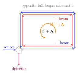
- Michelson 镜位移 \(x>0\) 定义为使该臂物理长度增加。Sagnac 先选有向面积 \(\mathbf A\);沿其右手边界方向传播的光定义为 \(+\) 束,反向为 \(-\) 束,并定义 \(\Delta\phi_{\mathrm S}=\phi_+-\phi_-\)。
- 本课不展开完整统计光学、量子相干、高阶相关或噪声谱估计,只建立一阶 coherence 和经典干涉测量。
Notation and modeling contract / 符号与建模契约
| Symbol | Meaning | SI unit |
|---|---|---|
| \(\Gamma_{12},\gamma_{12}\) | mutual coherence 与归一化 degree of coherence | \(\mathrm{V^2\,m^{-2}}\), 1 |
| \(\tau_c,l_c\) | coherence time 与 coherence length | s, m |
| \(A_c\) | transverse coherence area / 横向相干面积 | \(\mathrm{m^2}\) |
| \(\mathcal V\) | fringe visibility | 1 |
| \(\Delta,\delta\) | OPD 与相位差 | m, rad |
| \(x,l,n\) | 镜位移、样品长度、折射率 | m, m, 1 |
| \(\mathbf A,\boldsymbol\Omega\) | Sagnac 有向面积与角速度 | \(\mathrm{m^2}\), \(\mathrm{rad\,s^{-1}}\) |
Knowledge 1 — Temporal and spatial coherence / 时间与空间相干性
Knowledge ID: P05-U04-L03-K01
1.1 时间相干:同一场能“记住”多久
时间相干比较同一点场在相隔 \(\tau\) 的两个时刻:
\[\Gamma(\tau)=\left\langle E^*(t)E(t+\tau)\right\rangle.\]
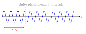
理想单色场的相位永不漂移,\(\lvert\gamma(\tau)\rvert=1\)。真实有限谱宽场由许多频率分量组成,延迟后它们相对相位逐渐散开,使 \(\lvert\gamma(\tau)\rvert\) 衰减。Wiener–Khinchin relation 表明一阶自相关与功率谱互为 Fourier transform;“窄谱对应长相干时间”不是口号,而是 Fourier 对偶。
1.2 空间相干:同一波前能“横向一致”多远
空间相干比较同一时刻不同位置 \(\mathbf r_1,\mathbf r_2\) 的场:
\[\Gamma(\mathbf r_1,\mathbf r_2) =\left\langle E^*(\mathbf r_1,t)E(\mathbf r_2,t)\right\rangle.\]
远处小角源的不同源点产生不同横向波矢;当两采样点间距增加,各源点贡献的相位差分散,条纹变淡。van Cittert–Zernike theorem 把远场 mutual coherence 与非相干源的角强度分布联系起来。数量级上,若源角宽为 \(\alpha\),
\[\ell_{\mathrm{coh}}\sim\frac{\lambda}{\alpha},\]
但精确系数取决于源形状和 coherence width 的定义。
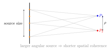
时间与空间相干不是两种光;它们是同一随机场沿不同变量切片的相关性。实验装置可同时受二者限制。
Knowledge 2 — Coherence time, length, and area / 相干时间、长度与面积
Knowledge ID: P05-U04-L03-K02
2.1 必须把“宽度定义”和“谱线形状”说清楚
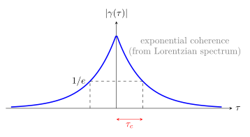
一种常用定义是:\(\tau_c\) 为 \(\lvert\gamma(\tau)\rvert\) 降到 \(1/e\) 的延迟。若功率谱是 Lorentzian,FWHM 为 \(\Delta\nu\),则
\[\lvert\gamma(\tau)\rvert =e^{-\pi\Delta\nu\lvert\tau\rvert}, \qquad \tau_c=\frac{1}{\pi\Delta\nu}.\]
真空 coherence length 为
\[l_c=c\tau_c.\]
若采用积分定义、半高定义或 Gaussian 谱,数值因子不同。因此只写 \(l_c=c/\Delta\nu\) 而不声明 convention 只能作为数量级估计。
2.2 相干面积
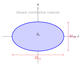
若横向相关在 \(x,y\) 两方向的特征宽度为 \(\ell_{cx},\ell_{cy}\),数量级上
\[A_c\sim \ell_{cx}\ell_{cy}.\]
圆对称情况下常写 \(A_c\sim\pi\ell_c^2\),但“半径”取 \(1/e\)、半高或第一零点会给不同面积。实验报告必须说明阈值和所用相关函数。
Knowledge 3 — Fringe visibility and mutual coherence / 条纹可见度与互相干性
Knowledge ID: P05-U04-L03-K03
3.1 一般双束强度
两束场在探测器叠加,延迟为 \(\tau\),外加可扫描相位 \(\phi\)。时间平均强度为
\[I(\phi,\tau) =I_1+I_2 +2\sqrt{I_1I_2} \operatorname{Re}\!\left[\gamma_{12}(\tau)e^{i\phi}\right].\]
扫描 \(\phi\) 得
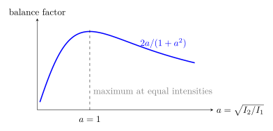
\[\mathcal V =\frac{I_{\max}-I_{\min}}{I_{\max}+I_{\min}} =\frac{2\sqrt{I_1I_2}}{I_1+I_2} \lvert\gamma_{12}(\tau)\rvert.\]
因此可见度是“强度平衡因子”与“相干度”的乘积。若不先测 \(I_1,I_2\),不能把 \(\mathcal V\) 直接当成 \(\lvert\gamma_{12}\rvert\)。
3.2 如何测量 mutual coherence
- 改变 delay 并记录 \(\mathcal V(\tau)\):得到 temporal coherence envelope。
- 改变两个采样孔的横向间距并记录 \(\mathcal V(\rho)\):得到 spatial coherence。
- 每个 delay 先分别遮挡两臂测 \(I_1,I_2\),再除去强度平衡因子。
- 有限像素、振动、相位扫描非线性和背景光都会偏置极值,必须纳入不确定度。
Knowledge 4 — Michelson, Mach–Zehnder, and Sagnac interferometers / 三类典型干涉仪
Knowledge ID: P05-U04-L03-K04
4.1 Michelson:紧凑双程、对位移敏感
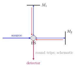
一个 beamsplitter 把光分到相互垂直的两臂,镜面反射后返回并重合。镜位移 \(x\) 改变往返 OPD \(2x\)。补偿片可使两束通过相近玻璃厚度,减小色散差。
4.2 Mach–Zehnder:分离单程路径、适合放置样品
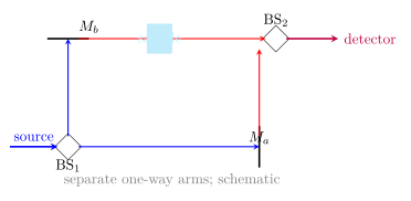
两个 beamsplitter 和两个 mirrors 形成分开的两条单程路径,再在第二分束器合束。样品可只置于 signal arm,便于成像或流场测量;但非公共路径使它对振动和空气扰动更敏感。
4.3 Sagnac:反向共路、对旋转敏感
同一 beamsplitter 产生 \(+\) 与 \(-\) 两束,它们沿同一闭合路径反向传播;选定 \(\mathbf A\) 后,\(+\) 束沿其右手边界方向。静止互易扰动多为 common mode;装置旋转时两束传播时间不同。定义 \(\Delta t=t_+-t_-\),则真空中、低速极限:
\[\Delta t=t_+-t_- =\frac{4\mathbf A\cdot\boldsymbol\Omega}{c^2},\]
\[\Delta\phi_{\mathrm S} =\phi_+-\phi_- =\omega\Delta t =\frac{8\pi\mathbf A\cdot\boldsymbol\Omega}{\lambda_0c}.\]
Knowledge 5 — Precision displacement and index measurement / 精密位移与折射率测量
Knowledge ID: P05-U04-L03-K05
5.1 位移与相位
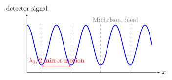
Michelson 中镜位移 \(x\) 使 OPD 变化 \(2x\):
\[\Delta\phi=\frac{4\pi x}{\lambda_0}, \qquad x=\frac{\lambda_0\Delta\phi}{4\pi}.\]
若只数完整条纹 \(N\),
\[x=\frac{N\lambda_0}{2}.\]
相位拟合允许测量小于一整条纹的位移,但“亚波长分辨率”不等于“亚波长准确度”;系统误差仍受波长真空/空气换算、cosine error、Abbe error、相位非线性和温漂控制。
5.2 折射率
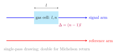
长度 \(l\) 的气室从真空变为折射率 \(n\):
- Mach–Zehnder 单程:\(\Delta=(n-1)l\)。
- Michelson 气室被往返穿过:\(\Delta=2(n-1)l\)。
对应完整条纹计数分别为
\[N_{\mathrm{MZ}}=\frac{(n-1)l}{\lambda_0}, \qquad N_{\mathrm{Mich}}=\frac{2(n-1)l}{\lambda_0}.\]
5.3 测量链与不确定度

图 11 提醒:干涉仪直接输出相位或强度,不直接输出“真实长度”。从相位到物理量必须经过模型、校准和不确定度传播。
Worked Examples / 完整例题
Worked Example 1 — 由 Lorentzian 线宽求相干时间与长度
已知: 光源功率谱为 Lorentzian,FWHM \(\Delta\nu=1.00\,\mathrm{GHz}\)。采用 \(\lvert\gamma\rvert=1/e\) 定义 \(\tau_c\),在真空中传播。
研究对象与参考系: 实验室中同一场的延迟自相关;延迟正负对模长相同。
模型理由: 已明确 Lorentzian 线形和 \(1/e\) amplitude convention。
\[\tau_c=\frac{1}{\pi\Delta\nu} =\frac{1}{\pi(1.00\times10^9)} =3.18\times10^{-10}\,\mathrm s.\]
\[l_c=c\tau_c =(2.9979\times10^8)(3.18\times10^{-10}) =9.54\times10^{-2}\,\mathrm m.\]
结果: \(\tau_c=0.318\,\mathrm{ns}\),\(l_c=95.4\,\mathrm{mm}\)。
检查与解释: \(\Delta\nu\tau_c\) 无量纲;线宽趋零时相干时间趋无穷。若改用 Gaussian 谱或 FWHM correlation 定义,数值因子会改变,不能无说明比较。
Worked Example 2 — 从 visibility 分离强度失配与相干度
已知: \(I_1=9.00\,\mathrm{W\,m^{-2}}\)、\(I_2=4.00\,\mathrm{W\,m^{-2}}\),扫描相位测得 \(\mathcal V=0.700\)。求 \(\lvert\gamma_{12}\rvert\)。
系统: 固定探测器收集同偏振同频带两束光;背景已扣除。
模型理由: 相位扫描覆盖极大和极小,强度在扫描中稳定。
\[\lvert\gamma_{12}\rvert =\mathcal V\frac{I_1+I_2}{2\sqrt{I_1I_2}} =0.700\frac{13.00}{12.00} =0.758.\]
检查与解释: 结果满足 \(0\le\lvert\gamma\rvert\le1\)。若错误地把 \(\mathcal V\) 直接当 \(\lvert\gamma\rvert\),会把强度失配造成的损失也归因于失相干。
Worked Example 3 — Michelson 条纹计数测镜位移
已知: \(\lambda_0=632.8\,\mathrm{nm}\),镜面缓慢移动时有 \(N=237\) 个完整条纹通过固定参考点。
研究对象与方向: Michelson 可动镜;正方向取臂长增加。
模型理由: 镜移动造成双程 OPD \(2x\);空气折射率变化和相位漏计忽略。
\[x=\frac{N\lambda_0}{2} =\frac{237(632.8\,\mathrm{nm})}{2} =74.99\,\mu\mathrm m.\]
检查与解释: 每个条纹对应镜移动 \(\lambda_0/2=316.4\,\mathrm{nm}\),数量级一致。若镜沿光轴反向移动,位移带负号但计数绝对值相同。四位有效数字反映给定波长和整数计数,不代表未计入的系统误差。
Worked Example 4 — Sagnac 环的旋转相位
已知: 单圈平面环面积 \(A=0.250\,\mathrm{m^2}\),法向与角速度同向,\(\Omega=0.500\,\mathrm{rad\,s^{-1}}\),\(\lambda_0=632.8\,\mathrm{nm}\)。
系统与参考系: 随装置旋转的闭合真空光路;低速 \(v_{\mathrm{rim}}\ll c\)。
方向: 按本课约定,\(+\) 束沿 \(\mathbf A\) 的右手边界方向传播,且 \(\Delta\phi_{\mathrm S}=\phi_+-\phi_-\)。这里 \(\mathbf A\cdot\boldsymbol\Omega>0\),所以 \(+\) 束与装置同向旋转、传播时间较长,故相位差为正。
\[\Delta\phi_{\mathrm S} =\frac{8\pi A\Omega}{\lambda_0c} =\frac{8\pi(0.250)(0.500)} {(632.8\times10^{-9})(2.9979\times10^8)} =1.66\times10^{-2}\,\mathrm{rad}.\]
检查与解释: 相位无量纲;\(A\to0\) 或 \(\Omega\to0\) 时信号消失,反转旋转方向时符号反转。单圈相位很小,实际 fiber gyro 通过多圈有效面积和锁相读出增强灵敏度。
Lesson synthesis / 本课综合
- 先定义比较对象: 时间延迟、横向间距或两条仪器路径。
- 选择相关函数: \(\Gamma_{12}\) 给绝对交叉强度,\(\gamma_{12}\) 给归一化相干度。
- 预测可见度: 把强度平衡因子与 \(\lvert\gamma_{12}\rvert\) 分开。
- 选择拓扑: Michelson 适合紧凑双程位移;Mach–Zehnder 适合单程样品与成像;Sagnac 适合反向共路的非互易相位。
- 画路径并算 OPD: 明确单程/双程、分束器相位和样品通过次数。
- 把相位反演为物理量: 同时传播波长、相位拟合、环境和几何不确定度。
Formula-and-decision table / 公式与决策表
| Question | Equation / model | Use only when | Key warning |
|---|---|---|---|
| 一阶相干怎么定义? | \(\Gamma_{12}(\tau)=\langle E_1^*(t)E_2(t+\tau)\rangle\) | 场统计平稳或平均窗口合理 | 共轭位置决定相位符号 |
| 相干度? | \(\gamma_{12}=\Gamma_{12}/\sqrt{\Gamma_{11}\Gamma_{22}}\) | 分母非零 | \(\lvert\gamma\rvert\le1\) |
| visibility 与 coherence? | \(\mathcal V=\frac{2\sqrt{I_1I_2}}{I_1+I_2}\lvert\gamma_{12}\rvert\) | 能扫描相位且背景已校正 | 先测单臂强度 |
| Lorentzian \(\tau_c\)? | \(\tau_c=1/(\pi\Delta\nu)\) | FWHM line width、\(1/e\) amplitude 定义 | 换线形或定义会换因子 |
| Michelson 位移? | \(x=\lambda_0\Delta\phi/(4\pi)=N\lambda_0/2\) | 镜沿光轴、双程 | 空气波长和 cosine error |
| MZ 折射率? | \(N=(n-1)l/\lambda_0\) | 单程样品 | Michelson 往返多因子 2 |
| Sagnac 相位? | \(\Delta\phi=8\pi\mathbf A\cdot\boldsymbol\Omega/(\lambda_0c)\) | 低速、闭合光路、单圈 | 多圈使用有效有向面积和 |
Model boundaries / 模型边界
- 平稳统计: 若光源或装置在平均窗口内显著漂移,时间平均不等于稳定系综平均。
- 一阶 coherence: \(\gamma_{12}\) 描述强度干涉;非经典光和 photon correlations 需要更高阶相关。
- 谱宽—相干长度: 必须给出谱线形状和宽度定义;多峰谱可出现 coherence revival,不能只用一个 \(l_c\)。
- 空间 coherence: \(\ell\sim\lambda/\alpha\) 是数量级;精确轮廓由源强度分布的 Fourier transform 决定。
- 仪器拓扑: 实际 beamsplitter 有偏振、色散和附加相位;不对称损耗改变输出端口关系。
- metrology: 相位分辨率不是准确度。波长溯源、空气折射率、热膨胀、Abbe/cosine error、电子非线性都可主导误差。
- Sagnac: 给出的式子是低速真空单圈结果;运动介质、非平面回路和相对论精密模型需更完整处理。
Misconception clinic / 误区诊所
- “看得到条纹就叫完全相干。” 任意非零 \(\lvert\gamma\rvert\) 都可能给条纹;完全相干要求归一化模为 1,且还要校正强度失配。
- “coherence length 永远是 \(c/\Delta\nu\)。” 数值因子取决于谱线形状、FWHM 或 RMS 宽度以及 coherence threshold。
- “时间相干差就是空间相干差。” 它们分别沿时间延迟与空间分离测量;同一源可在一方面好、另一方面差。
- “Michelson 镜移动一波长只走一条条纹。” 往返 OPD 变化 \(2\lambda\),会走两条条纹。
- “Sagnac 两束走同一路,所以永远零相位差。” 静止互易扰动近似共模;旋转使反向传播时间不同,正是信号来源。
- “能拟合到 \(10^{-3}\) 条纹就有 \(10^{-3}\lambda\) 准确度。” 这只描述读出分辨率;系统校准和环境偏差可能大得多。
Practice and retrieval / 练习与提取
- K01: temporal coherence 比较什么?spatial coherence 又比较什么?
Answer
前者比较同一场在不同时刻或路径延迟下的相关;后者比较同一时刻不同横向位置的相关。
- K02: Lorentzian 线宽 \(\Delta\nu=5.00\,\mathrm{MHz}\),按本课 \(1/e\) 定义求真空 \(l_c\)。
Answer
\[l_c=\frac{c}{\pi\Delta\nu} =19.1\,\mathrm m.\]
- K02: 源的角宽加倍而波长不变,横向 coherence width 数量级怎样变?
Answer
由 \(\ell_{\mathrm{coh}}\sim\lambda/\alpha\),约减半;精确系数仍取决于源形状与宽度定义。
- K03: 等强双束测得 visibility \(0.62\),背景已扣除。求 \(\lvert\gamma_{12}\rvert\)。
Answer
等强时平衡因子为 1,所以 \(\lvert\gamma_{12}\rvert=0.62\)。
- K03: 完全相干但强度比 \(I_2/I_1=1/9\),最大 visibility 是多少?
Answer
振幅比 \(a=1/3\),故 \(\mathcal V=2a/(1+a^2)=0.600\)。
- K04/K05: Michelson 中镜移动 \(12.0\,\mu\mathrm m\),\(\lambda_0=600\,\mathrm{nm}\)。经过多少条纹?
Answer
\(N=2x/\lambda_0=40.0\)。
- K05: Mach–Zehnder 一臂中长 \(l=10.0\,\mathrm{mm}\) 的气室产生 \(N=4.00\) 条纹,\(\lambda_0=500\,\mathrm{nm}\)。求 \(n\)。
Answer
\(n=1+N\lambda_0/l=1.000200\)。
- K04: 上题气室若放入 Michelson 并被往返穿过,其他条件不变,会走多少条纹?
Answer
OPD 加倍,因此为 \(8.00\) 条纹。
- K04: 反转 Sagnac 环面积矢量而保持 \(\boldsymbol\Omega\) 不变,输出相位怎样变?
Answer
\(\mathbf A\cdot\boldsymbol\Omega\) 变号,所以 \(\Delta\phi_{\mathrm S}\) 变号,大小不变。
- 综合: 扫描 delay 时 visibility 降低,但两臂单独强度也随 delay 改变。怎样提取真正的 \(\lvert\gamma_{12}(\tau)\rvert\)?
Answer
每个 delay 分别测 \(I_1(\tau),I_2(\tau)\) 和条纹极值,先求 \(\mathcal V(\tau)\),再除以 \(2\sqrt{I_1I_2}/(I_1+I_2)\);还应扣除背景并传播强度不确定度。
Exit ticket / 离堂检核
- 设计一个实验区分“有限线宽导致的 temporal decoherence”和“机械振动导致的 visibility 降低”,明确要扫描的变量和预期函数形状。
- 为 \(100\,\mathrm{nm}\) 量级位移测量在 Michelson、Mach–Zehnder、Sagnac 中选一种拓扑;说明选择理由、相位—位移关系及前三项系统误差。
References and source notes / 参考资料与来源说明
Source-to-content map
| Source | Used for | Knowledge ID / section | Model boundary or convention |
|---|---|---|---|
| OpenStax University Physics Vol. 3, 3.5 The Michelson Interferometer | Michelson paths, factor of two, displacement and index measurement | K04–K05 | mirror motion changes round-trip OPL |
| MIT OCW 2.71, Lecture 15 | Michelson/Mach–Zehnder layouts, visibility and phase metrology | K03–K05 | detector averages intensity rather than optical field |
| MIT OCW 2.71, Lecture 22: Coherent and Incoherent Imaging | temporal/spatial coherence and correlation functions | K01–K03 | coherence width convention stated |
| MIT OCW 2.71 (2014), Lecture 11 Notes on Wave Optics | Michelson autocorrelation and Young spatial-correlation interpretation | K01–K03 | normalized coherence separated from intensity imbalance |
| Rutgers Physics, Sagnac Interferometer Theory and Background | counter-propagating loop, rotation phase and beamsplitter phases | K04 | low-speed, closed-loop orientation convention |
| NIST, Realizing Pressure, Temperature, and Length | practical Fabry–Pérot refractive-index/displacement metrology | K05 | calibration and uncertainty chain, not ideal fringe count alone |
资料与 URL 实际打开核对日期:2026-08-28。正文重新组织;所有图依据方程原创绘制;数值例题与练习独立复算。
复习与拓展
- Huygens–Fresnel diffraction:孔径不同位置的空间相干决定可否作场的相干积分。
- Fourier Optics:mutual intensity 与 coherent/incoherent transfer functions。
- Laser linewidth and cavities:腔模、线宽与 temporal coherence 的来源。
- 实验接口:phase unwrapping、quadrature detection、Allan deviation、空气折射率补偿和 SI-traceable wavelength。