
Learning objectives / 学习目标
完成本课后,你应能:
- 从有限宽度、有限数量、等间距狭缝的相量和推导“单缝 envelope × \(N\)-slit interference factor”。
- 判定 principal maxima、次极大、零点与 missing orders,并说明增加 illuminated grooves 为何使峰变窄。
- 在明确 signed-angle convention 后使用一般 grating equation,并检查可传播级次条件。
- 推导 angular dispersion \(d\theta/d\lambda\) 与理想 resolving power \(\mathcal R=\lvert m\rvert N\),区分分散与分辨。
- 建立从 entrance slit、collimator、grating、camera、detector 到 wavelength/radiometric calibration 的真实光谱测量链。
Prerequisites / 先修知识
- 双源相位与条纹。
- 单缝 sinc-squared envelope。
- 等比级数、复相量、微分、Rayleigh-type resolution criterion。
Scope and conventions / 范围与约定
- \(N\) 个相同狭缝,每缝宽 \(a\),相邻中心距 \(d\),通常 \(d>a\);均匀相干正入射。
- 传播介质均匀,波长为 \(\lambda\)。若给真空波长,先除以折射率。
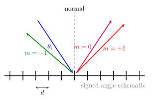
- 正入射时观察角 \(\theta\) 从光栅法线测量。一般入射采用 signed transverse-wavevector convention:
\[d(\sin\theta_m-\sin\theta_i)=m\lambda.\]
若教材把入射、出射角在法线两侧都取正数,式子会写成加号;物理内容是横向波矢差。
- groove density \(g\) 以 \(\mathrm{m^{-1}}\) 或 lines/mm 给出,周期 \(d=1/g\)。
- 理想分辨本领 \(\mathcal R=\lvert m\rvert N\) 假设衍射极限、均匀照明、无像差、窄入口缝和足够采样。
Notation and modeling contract / 符号与建模契约
| Symbol | Meaning | SI unit |
|---|---|---|
| \(a,d,N\) | slit width, center spacing, illuminated slit count | m, m, 1 |
| \(\alpha=\pi a\sin\theta/\lambda\) | single-slit phase parameter | 1 |
| \(\beta=\pi d\sin\theta/\lambda\) | adjacent-slit half phase difference | 1 |
| \(m\) | diffraction order | 1 |
| \(g=1/d\) | groove density | \(\mathrm{m^{-1}}\) |
| \(\mathcal D=d\theta/d\lambda\) | angular dispersion | \(\mathrm{rad\,m^{-1}}\) |
| \(\mathcal R=\lambda/\Delta\lambda\) | resolving power | 1 |
Knowledge 1 — Combined interference and diffraction envelope / 干涉与衍射包络
Knowledge ID: P05-U05-L02-K01
1.1 两个尺度、两个因子
单个宽 \(a\) 的狭缝给振幅因子 \(\sin\alpha/\alpha\)。\(N\) 个中心间距 \(d\) 的等间距缝,其相邻缝相位差为 \(2\beta\),几何级数给阵列振幅
\[\sum_{q=0}^{N-1}e^{i2q\beta} =e^{i(N-1)\beta}\frac{\sin(N\beta)}{\sin\beta}.\]
将强度归一化到中央峰:
\[\frac{I(\theta)}{I(0)} = \left(\frac{\sin\alpha}{\alpha}\right)^2 \left(\frac{\sin(N\beta)}{N\sin\beta}\right)^2,\]
\[\alpha=\frac{\pi a\sin\theta}{\lambda}, \qquad \beta=\frac{\pi d\sin\theta}{\lambda}.\]
第一个因子是 single-slit envelope,第二个是 finite-array interference factor。它们相乘,不是相加。
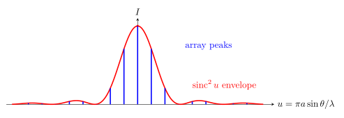
图 1 是结构示意,不用离散竖线代替真实有限宽峰;它强调每个 grating peak 的可用强度受 envelope 限制。
1.2 Principal maxima、零点与峰宽
当 \(\beta=m\pi\) 时所有缝同相:
\[d\sin\theta_m=m\lambda.\]
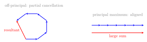
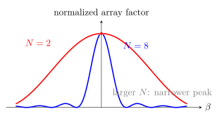
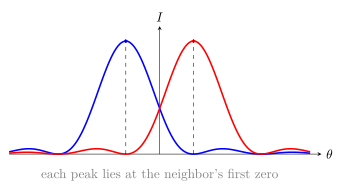
在相邻 principal maxima 之间,array factor 有 \(N-1\) 个零点和 \(N-2\) 个较弱次极大。principal maximum 附近第一零点满足
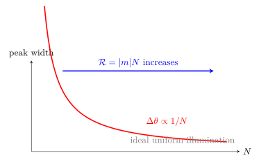
\[\Delta(\sin\theta)\approx\frac{\lambda}{Nd},\]
所以 \(N\) 越大,峰越窄、峰值越高;总能量仍由完整角积分和 aperture throughput 守恒。
1.3 Missing orders
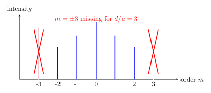
若某 principal grating maximum 同时落在 single-slit minimum,则该级缺失:
\[d\sin\theta=m\lambda, \qquad a\sin\theta=p\lambda.\]
合并为
\[ma=pd.\]
例如 \(d/a=3\) 时,\(m=3,6,9,\ldots\) 与单缝零点重合。所谓 missing order 是 envelope 把该阵列峰乘成零,并非 grating equation 失效。
Knowledge 2 — Diffraction-grating equation / 衍射光栅方程
Knowledge ID: P05-U05-L02-K02
2.1 横向波矢匹配
周期结构只允许横向波矢相差 reciprocal-lattice multiples:
\[k\sin\theta_m-k\sin\theta_i=\frac{2\pi m}{d}.\]
故 signed-angle grating equation 为
\[d(\sin\theta_m-\sin\theta_i)=m\lambda.\]
正入射 \(\theta_i=0\) 时:
\[d\sin\theta_m=m\lambda.\]
可传播级次必须满足 \(\lvert\sin\theta_m\rvert\le1\)。反射/透射 grating、角度取正方式或 groove blaze 会改变符号书写和各级效率,但不会改变横向动量匹配。
2.2 Groove density 与 order overlap
若 groove density 为 \(g\) lines per unit length,
\[d=\frac1g.\]
同一方向可满足
\[m\lambda=m'\lambda',\]
因此不同 order 的不同波长可重叠。真实光谱仪常用 order-sorting filter、cross-disperser 或限制波段来消除歧义。
Knowledge 3 — Angular dispersion and resolving power / 角色散与分辨本领
Knowledge ID: P05-U05-L02-K03
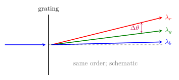
3.1 Angular dispersion
正入射 grating equation 对 \(\lambda\) 微分:
\[d\cos\theta_m\,d\theta_m=m\,d\lambda.\]
所以
\[\mathcal D =\frac{d\theta_m}{d\lambda} =\frac{m}{d\cos\theta_m}.\]
较高 order、较小 period 或接近 grazing angle 会提高 angular dispersion。高 dispersion 只说明波长映射角度更分开;若线宽、入口缝像或像差同样很宽,仍未必能分辨。
3.2 Resolving power
理想均匀光栅 illuminated grooves 数为 \(N\)。相邻波长满足 Rayleigh-type just-resolution 时,
\[\mathcal R =\frac{\lambda}{\Delta\lambda} =\lvert m\rvert N.\]
更高 order 和更多 illuminated grooves 提高 diffraction-limited resolving power。这里 \(N\) 是实际被照亮且有效相干的 groove 数,不一定是整块光栅标称总 groove 数。
Knowledge 4 — Spectroscopy with gratings / 光栅光谱学
Knowledge ID: P05-U05-L02-K04
4.1 光谱仪不是“光栅加屏幕”
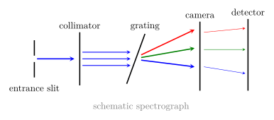
典型 spectrograph:
- entrance slit 定义被测空间区域和几何线宽;
- collimator 把光变为近似平面波;
- grating 按波长分散;
- camera optic 把角度映射到 detector position;
- detector 采样并引入 pixel response、read noise 和背景;
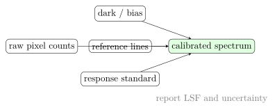
- reference lines 建立 wavelength calibration,标准辐射源建立 spectral-response calibration。
4.2 仪器线形与校准
detector 上测到的 spectrum 可概念性写为
\[C(p) =\int S(\lambda)\, H\!\left[p-p(\lambda)\right]\, \eta(\lambda)\,d\lambda+B(p),\]
其中 \(S\) 是真实谱,\(H\) 是 instrument line-spread function,\(\eta\) 是 spectral response,\(B\) 是背景。波长校准只确定 \(p\leftrightarrow\lambda\);它不自动校正 \(\eta(\lambda)\),也不消除 stray light 或 saturation。
4.3 实际分辨率的限制
理想 \(\lvert m\rvert N\) 只是上限。真实 \(\Delta\lambda_{\mathrm{inst}}\) 还受:
- entrance slit width 与像差;
- illuminated footprint 和 apodization;
- detector pixel sampling 与 charge spread;
- grating figure/groove errors;
- source line width、defocus、stray light 与 signal-to-noise;
- wavelength model 残差与温度漂移。
至少约两个 detector samples 才能表示一个线形宽度;“像素更小”也不会突破光学 line-spread function。
Worked Examples / 完整例题
Worked Example 1 — 双尺度图样与 missing order
已知: \(a=20.0\,\mu\mathrm m\),\(d=60.0\,\mu\mathrm m\),\(\lambda=600\,\mathrm{nm}\),正入射。求前三个正级 principal angles,并判定缺级。
系统与坐标: 均匀相干多缝,\(\theta>0\) 为屏上正方向。
模型理由: Fraunhofer、小角但先用精确 \(\sin\theta\);缝宽相同。
\[\sin\theta_m=\frac{m\lambda}{d}=0.0100m.\]
所以
\[\theta_1=0.573^\circ,\qquad \theta_2=1.15^\circ,\qquad \theta_3=1.72^\circ.\]
但 \(d/a=3\)。在 \(m=3\) 时
\[a\sin\theta_3 =a\frac{3\lambda}{d} =\lambda,\]
正好是单缝第一极小,因此第 3 级缺失。
检查与解释: 所有 \(\sin\theta<1\);缺级来自 envelope 零点,而非 grating equation 无解。更高的 \(m=6,9,\ldots\) 也按同一比例缺失,前提是它们可传播。
Worked Example 2 — 光栅角位置与角色散
已知: \(g=1200\,\mathrm{lines/mm}\),正入射,\(\lambda=500\,\mathrm{nm}\),\(m=1\)。
研究对象: 一阶 transmitted diffraction direction;角度相对法线为正。
模型理由: 均匀介质、标量 grating equation。
\[d=\frac{1}{1.200\times10^6} =8.333\times10^{-7}\,\mathrm m.\]
\[\sin\theta_1=\frac{500\times10^{-9}}{8.333\times10^{-7}}=0.600, \qquad \theta_1=36.9^\circ.\]
\[\mathcal D =\frac{1}{d\cos\theta_1} =\frac{1}{(8.333\times10^{-7})(0.800)} =1.50\times10^6\,\mathrm{rad\,m^{-1}} =1.50\times10^{-3}\,\mathrm{rad\,nm^{-1}}.\]
检查与解释: dispersion 单位是 rad/length;增加 \(m\) 或接近 grazing 可提高它,但 blaze efficiency 和 order overlap 仍需检查。
Worked Example 3 — 理想光栅能分开多近的谱线
已知: illuminated grooves \(N=25\,000\),二阶 \(m=2\),中心波长 \(\lambda=600.0\,\mathrm{nm}\)。
系统与边界: 理想均匀衍射极限 grating;入口缝、像差和 detector 不限制。
模型理由: 使用 Rayleigh-type \(\mathcal R=\lvert m\rvert N\)。
\[\mathcal R=\lvert m\rvert N =\lvert2\rvert(25\,000) =50\,000.\]
\[\Delta\lambda_{\min} =\frac{\lambda}{\mathcal R} =\frac{600.0\,\mathrm{nm}}{50\,000} =0.0120\,\mathrm{nm}.\]
检查与解释: \(\Delta\lambda\) 与 \(\lambda\) 同单位且远小于中心波长。这个值是理想下限;若 entrance slit 或 LSF 对应 \(0.050\,\mathrm{nm}\),实际分辨率只能约 \(0.050\,\mathrm{nm}\)。
Worked Example 4 — 两点波长校准与仪器采样
已知: 参考线 \((p_1,\lambda_1)=(400,500.0\,\mathrm{nm})\)、\((p_2,\lambda_2)=(1400,600.0\,\mathrm{nm})\)。未知峰在 \(p=875\),局部 LSF FWHM 为 3.0 pixels。
研究对象: detector 一维 dispersion axis;像素编号向长波方向增加。
模型理由: 只在此窄区采用线性 wavelength model;两参考线无误识别。
斜率
\[\frac{d\lambda}{dp} =\frac{600.0-500.0}{1400-400} =0.1000\,\mathrm{nm/pixel}.\]
\[\lambda(875) =500.0+(875-400)(0.1000) =547.5\,\mathrm{nm}.\]
instrumental FWHM 为
\[\Delta\lambda_{\mathrm{inst}} =(3.0)(0.1000)=0.30\,\mathrm{nm}.\]
检查与解释: 未知点位于两参考点之间,是插值而非外推;三像素宽满足基本采样。实际报告还需拟合残差、参考线不确定度和 response calibration,不能仅报计算波长。
Lesson synthesis / 本课综合
- 写 aperture transmission:单缝宽度 \(a\) 与阵列位置 \(qd\) 是两个独立尺度。
- 对单缝积分得到 envelope;对 \(N\) 个中心作几何级数得到 array factor。
- 用 \(d\sin\theta=m\lambda\) 找 principal directions,再检查单缝零点是否制造 missing order。
- 用峰旁第一零点估计角宽;由 grating equation 微分求 dispersion。
- 用 \(\mathcal R=\lvert m\rvert N\) 得 diffraction-limited 上限,再与入口缝像、像差、LSF 和像素采样比较。
- 在光谱测量中分开 wavelength calibration、spectral-response calibration 和 uncertainty validation。
Formula-and-decision table / 公式与决策表
| Question | Equation / model | Use only when | Key warning |
|---|---|---|---|
| 完整 \(N\)-slit 图样? | sinc-squared envelope × normalized array factor | identical, uniformly illuminated slits | 两因子相乘 |
| Principal maxima? | \(d\sin\theta_m=m\lambda\) | 正入射 signed angle | 还要检查 envelope |
| Missing order? | \(ma=pd\) | grating peak 与 slit zero 重合 | 不是 grating equation 无解 |
| 一般入射? | \(d(\sin\theta_m-\sin\theta_i)=m\lambda\) | 本课 signed convention | 其他角号约定可能写加号 |
| 可传播级次? | \(\lvert\sin\theta_m\rvert\le1\) | 均匀传播介质 | grazing 级通常难收集 |
| Angular dispersion? | \(d\theta/d\lambda=m/(d\cos\theta_m)\) | 固定 order、正入射 | dispersion 不等于 resolution |
| Ideal resolving power? | \(\mathcal R=\lvert m\rvert N\) | diffraction-limited grating | \(N\) 是实际 illuminated grooves |
| Detector spectrum? | true spectrum convolved with LSF and multiplied by response | linear detector、calibrated model | 波长校准不等于响应校准 |
Model boundaries / 模型边界
- 标量薄光栅: blaze、深沟槽、偏振和 vector electromagnetic coupling 会改变 efficiency;本课式子主要给角位置。
- 均匀照明: apodization 降低旁瓣但加宽主峰,理想 \(\lvert m\rvert N\) 的线形需修正。
- 有限 coherence: illuminated grooves 若不能相干叠加,有效 \(N\) 小于几何 groove 数。
- 入口缝: 真实 spectrograph 常在 slit-limited 而非 grating-limited regime。
- 高 order: order overlap、blaze envelope 和 detector bandpass 限制可用波段。
- 校准: 非线性 dispersion 需要多项式或物理模型;两点线性校准只适合局部。
Misconception clinic / 误区诊所
- “多缝图样就是很多单缝图样相加。” 相干场先相加;阵列因子与单缝 envelope 在强度中相乘。
- “光栅主峰都一样高。” 单缝 envelope、blaze、材料和偏振使各级效率不同。
- “missing order 表示没有满足 grating equation。” 它满足阵列同相条件,却同时落在单缝零点。
- “groove density 越大,任何波长的 order 越多。” 周期越小反而使 \(\lvert m\lambda/d\rvert\le1\) 更严格,可传播 order 数减少。
- “dispersion 大就一定 resolution 高。” resolution 还取决于峰宽、illuminated grooves、slit、像差和采样。
- “做了 wavelength calibration 就得到真实光谱强度。” 还需 dark/bias、spectral response、stray light 和线性校正。
Practice and retrieval / 练习与提取
- K01: \(N\) 从 10 增为 100,理想 principal peak 的近邻第一零点间角宽约怎样变?
Answer
约缩小为原来的 \(1/10\),因为 \(\Delta\theta\propto1/N\)(同一 \(d,\lambda,\theta_m\))。
- K01: \(d/a=4\),哪些非零 grating orders 系统性缺失?
Answer
\(m=4,8,12,\ldots\) 及其负级,因为它们分别与单缝 \(p=1,2,3,\ldots\) 零点重合。
- K02: \(g=500\,\mathrm{lines/mm}\),求周期 \(d\)。
Answer
\(d=1/(5.00\times10^5)=2.00\,\mu\mathrm m\)。
- K02: 上题用 \(\lambda=600\,\mathrm{nm}\) 正入射,最高可传播整数 order 是多少?
Answer
\(\lvert m\rvert\le d/\lambda=3.33\),故最高 \(\lvert m\rvert=3\)。
- K02: 为什么同一角可能混合二阶 \(400\,\mathrm{nm}\) 与一阶 \(800\,\mathrm{nm}\)?
Answer
因为 \(m\lambda\) 相同:\(2(400)=1(800)\,\mathrm{nm}\),满足同一 grating angle。
- K03: \(d=1.00\,\mu\mathrm m\),\(m=1\),\(\theta=30^\circ\)。求 angular dispersion。
Answer
\[\mathcal D=\frac{1}{d\cos\theta} =1.15\times10^6\,\mathrm{rad\,m^{-1}} =1.15\times10^{-3}\,\mathrm{rad\,nm^{-1}}.\]
- K03: \(m=3\)、\(N=10\,000\),\(\lambda=450\,\mathrm{nm}\)。理想 \(\Delta\lambda\) 是多少?
Answer
\(\Delta\lambda=\lambda/(\lvert m\rvert N)=0.0150\,\mathrm{nm}\)。
- K04: optical LSF 为 2 pixels FWHM,但谱线只被 1 pixel 采样。主要问题是什么?
Answer
欠采样;像素无法可靠表示线形和峰位。应提高采样或改变 optical magnification,而不是仅依赖插值。
- K04: wavelength calibration 残差很小,是否证明 radiometric intensity 已准确?
Answer
否。波长映射与 spectral response 是不同校准;还需标准光源、暗场、线性和 stray-light 修正。
- 综合: 提高 entrance slit 宽度会怎样影响 throughput 与 spectral resolution?
Answer
通常 throughput 增加,但 slit image/LSF 变宽,分辨率下降;实际最优取决于 source size、SNR、grating limit 和 detector sampling。
Exit ticket / 离堂检核
- 设计一块 \(d/a=5\) 的多缝,画出前六级 principal peaks 与 single-slit envelope 的逻辑关系,并指出 missing orders。
- 给定 grating、camera focal length、pixel pitch 和 entrance slit width,建立从 \(\mathcal D\) 到 nm/pixel、再到实际 \(\Delta\lambda\) 的完整决策链。
References and source notes / 参考资料与来源说明
Source-to-content map
| Source | Used for | Knowledge ID / section | Model boundary or convention |
|---|---|---|---|
| OpenStax University Physics Vol. 3, 3.3 Multiple-Slit Interference | \(N\)-slit peaks, secondary maxima and narrowing | K01 | identical equally spaced slits |
| OpenStax University Physics Vol. 3, 4.3 Double-Slit Diffraction | interference factor under single-slit envelope and missing orders | K01 | Fraunhofer equal-slit model |
| OpenStax University Physics Vol. 3, 4.4 Diffraction Gratings | grating equation and qualitative dispersion | K02–K03 | normal incidence separated from general signed-angle form |
| UCL 1B24 Waves, Optics and Acoustics revision notes | exact diffraction-grating resolving-power relation, pp. 110–113 | K03 | source writes positive order \(m\); this lesson uses signed order and therefore \(\lvert m\rvert N\) |
| MIT OCW 2.71, Lecture 16: Gratings | amplitude/phase gratings, spatial periodicity and orders | K01–K02 | thin periodic transparency |
| MIT OCW 2.71, Lecture 17: Fraunhofer Diffraction | Fourier view of finite periodic apertures and peak width | K01–K03 | finite illuminated footprint |
| NIST High Resolution Atomic Spectroscopy | real grating spectrographs and wavelength standards | K04 | calibration and instrument line shape matter |
| NIST, Wavelength Calibration and Spectral Response Correction of CCD Array Spectrometers | wavelength/pixel and response calibration workflow | K04 | wavelength assignment and irradiance correction are distinct |
资料与 URL 实际打开核对日期:2026-08-28。正文重新组织;所有图依据方程原创绘制;数值例题与练习独立复算。
复习与拓展
- Resolution and Fourier Optics:finite periodic aperture 的 Fourier spectrum、convolution 与 transfer functions。
- Imaging Quality:spectrograph LSF 中 diffraction、aberration、slit 和 detector 的合成。
- Laser resonators:intracavity grating 与 wavelength selection。
- 实验接口:reference lamp line identification、polynomial wavelength fit、LSF deconvolution、order sorting 和 uncertainty budget。