
Learning objectives / 学习目标
- 从无限深方势阱边界条件推导 \(\phi_n(x)\)、\(E_n\) 与归一化常数。
- 用节点数、能级间距和一维非简并性解释量子数 \(n\) 的物理意义。
- 为中心有限方势阱写出 even/odd transcendental equations,并解释 evanescent tail。
- 用无量纲深度 \(z_0\) 图解并计数严格束缚态,同时识别阈值态不是可归一化束缚态。
- 计算能量本征态叠加的含时干涉项、Bohr frequency 与位置期望值。
Prerequisites / 先修知识
- Free Particles, Steps, and Barriers:传播波、倏逝解、\(\phi\) 与 \(\phi'\) 匹配。
- Schrödinger Equation:定态分离与 probability conservation。
- 三角函数正交性、定积分、复指数与 parity。
Scope and conventions / 范围与约定
- 单个无自旋、非相对论粒子;一维、实、时间无关势能;SI。
- 无限阱首先用 \(0<x<L\),外部 \(V=\infty\);因此 \(\phi(0)=\phi(L)=0\)。
- 有限阱统一用中心约定:\(V(x)=0\) for \(\lvert x\rvert<a\),\(V(x)=V_0>0\) for \(\lvert x\rvert\ge a\);阱宽为 \(2a\)。
- 有限阱束缚态满足 \(0<E<V_0\)。若把势能整体下移为阱内 \(-V_0\)、阱外 0,物理不变但能量零点改变。
- 对有限跳跃且质量恒定,\(\phi\) 与 \(\phi'\) 连续;无限墙是理想极限,墙外波函数为零。
- 本课不讨论 delta well、双阱隧穿劈裂、三维简并或数值 shooting algorithm 的实现细节。
Notation and modeling contract / 符号与建模契约
| Symbol | Meaning | SI unit |
|---|---|---|
| \(L\) | infinite-well width | m |
| \(a\) | finite-well half-width | m |
| \(V_0\) | exterior potential relative to well bottom | J |
| \(n\) | positive integer eigenstate label | 1 |
| \(k\) | interior oscillatory wavenumber \(\sqrt{2mE}/\hbar\) | \(\mathrm{m^{-1}}\) |
| \(\kappa\) | exterior decay constant \(\sqrt{2m(V_0-E)}/\hbar\) | \(\mathrm{m^{-1}}\) |
| \(z\) | dimensionless interior phase \(ka\) | 1 |
| \(z_0\) | dimensionless well strength \(a\sqrt{2mV_0}/\hbar\) | 1 |
| \(c_n\) | expansion amplitude in energy basis | 1 |
| \(\omega_{mn}\) | Bohr angular frequency \((E_m-E_n)/\hbar\) | \(\mathrm{s^{-1}}\) |
Knowledge 1 — Infinite square well / 无限深方势阱
Knowledge ID: P07-U03-L02-K01
阱内 \(V=0\) 的定态方程为
\[\frac{d^2\phi}{dx^2}+k^2\phi=0, \qquad k=\frac{\sqrt{2mE}}{\hbar}.\]
一般解 \(\phi=A\sin kx+B\cos kx\)。边界 \(\phi(0)=0\) 给 \(B=0\);\(\phi(L)=0\) 要求
\[\sin(kL)=0 \quad\Longrightarrow\quad kL=n\pi, \qquad n=1,2,3,\ldots.\]
归一化后
\[\phi_n(x)= \sqrt{\frac{2}{L}}\sin\left(\frac{n\pi x}{L}\right), \qquad 0<x<L,\]
墙外 \(\phi_n=0\)。
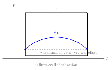
\(n=0\) 会给零函数,不能归一化;负 \(n\) 只改变整体符号,不产生新物理态。因此量子数从 1 开始。
Knowledge 2 — Energy quantization and nodes / 能量量子化与节点
Knowledge ID: P07-U03-L02-K02
允许波数离散,故能量为
\[E_n=\frac{\hbar^2k_n^2}{2m} =\frac{n^2\pi^2\hbar^2}{2mL^2}.\]
能量不是等间隔:
\[E_{n+1}-E_n=(2n+1)E_1.\]
第 \(n\) 个本征函数在阱内有 \(n-1\) 个节点。节点把波函数的符号区间分开,但节点处概率密度为零,不是粒子轨迹的反弹点。
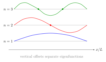
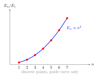
本征函数正交:
\[\int_0^L\phi_m^*(x)\phi_n(x)\,dx=\delta_{mn}.\]
一维实势的正规束缚态不简并。若两个同能量、可归一化解独立存在,它们的 Wronskian 为常数;无穷远或墙边界迫使该常数为零,于是两解线性相关。
Knowledge 3 — Finite square well and evanescent tails / 有限深方势阱与倏逝尾
Knowledge ID: P07-U03-L02-K03
有限中心阱取
\[V(x)= \begin{cases} 0, & \lvert x\rvert<a,\\ V_0, & \lvert x\rvert\ge a. \end{cases}\]
束缚态 \(0<E<V_0\) 在阱内振荡、阱外指数衰减:
\[k=\frac{\sqrt{2mE}}{\hbar}, \qquad \kappa=\frac{\sqrt{2m(V_0-E)}}{\hbar}, \qquad k^2+\kappa^2=\frac{2mV_0}{\hbar^2}.\]
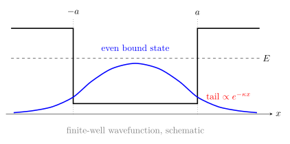
有限势阱中粒子不被严格限制在 \(\lvert x\rvert<a\);outside probability 是束缚态的一部分。\(E\to V_0^-\) 时 \(\kappa\to0\),尾巴变长,态接近连续谱阈值;\(V_0\to\infty\) 时 \(\kappa\to\infty\),尾巴消失并趋向无限阱。
Knowledge 4 — Bound-state counting and parity / 束缚态计数与宇称
Knowledge ID: P07-U03-L02-K04
因为 \(V(-x)=V(x)\),Hamiltonian 与 parity 对易;一维束缚态可选为 even 或 odd。定义
\[z=ka, \qquad z_0=a\frac{\sqrt{2mV_0}}{\hbar}, \qquad \kappa a=\sqrt{z_0^2-z^2}.\]
对 even state,阱内取 \(A\cos kx\);对 odd state,取 \(A\sin kx\)。在 \(x=a\) 匹配得到
\[z\tan z=\sqrt{z_0^2-z^2} \qquad \text{(even)},\]
\[-z\cot z=\sqrt{z_0^2-z^2} \qquad \text{(odd)}.\]
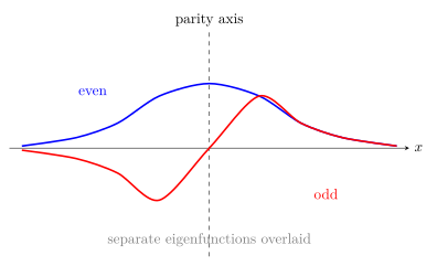
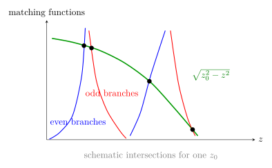
每一个交点对应一个束缚态。对 \(z_0>0\),严格束缚态总数可写成
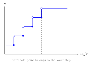
\[N=\left\lceil\frac{2z_0}{\pi}\right\rceil.\]
当 \(2z_0/\pi\) 恰为整数时,新解刚处于 \(E=V_0\),外侧 \(\kappa=0\),不是平方可积;上式的 ceiling 正好不把该阈值解算作新增束缚态。远离阈值时也可估算
\[N\sim\frac{2a\sqrt{2mV_0}}{\pi\hbar},\]
但近整数阈值必须回到 transcendental equations。
even ground state 对任意 \(V_0>0\) 都存在,这是“一维任意弱吸引势至少有一个束缚态”在方阱中的体现。激发态按 even、odd、even、odd 交替出现。
Knowledge 5 — Superpositions and time-dependent probability / 叠加态与含时概率
Knowledge ID: P07-U03-L02-K05
单个能量本征态
\[\psi_n(x,t)=\phi_n(x)e^{-iE_nt/\hbar}\]
只有整体相位随时间变,所以 \(\lvert\psi_n\rvert^2=\lvert\phi_n\rvert^2\) 静止。一般叠加
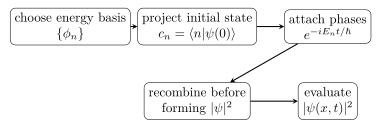
\[\psi(x,t)=\sum_n c_n\phi_n(x)e^{-iE_nt/\hbar}, \qquad \sum_n\lvert c_n\rvert^2=1\]
则密度含交叉项:
\[\lvert\psi\rvert^2 =\sum_n\lvert c_n\rvert^2\lvert\phi_n\rvert^2 +2\sum_{m>n}\operatorname{Re} \left[c_n^*c_m\phi_n^*\phi_m e^{-i(E_m-E_n)t/\hbar}\right].\]
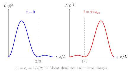
下图固定取 \(c_1=c_2=1/\sqrt2\)。在 \(t=0\) 与半拍频时刻 \(t=\pi/\omega_{21}\),相对相位由 \(+\) 翻为 \(-\),故
\[L\lvert\psi\rvert^2= \left[ \sin\left(\frac{\pi x}{L}\right) \pm\sin\left(\frac{2\pi x}{L}\right) \right]^2.\]
两幅密度严格关于 \(x=L/2\) 镜像,内部节点分别位于 \(2L/3\) 与 \(L/3\)。
时间依赖来自 relative phase;若所有占据分量同能量,密度仍静止。测量能量的概率 \(\lvert c_n\rvert^2\) 对时间不变,因为 Hamiltonian 本身不随时间变。
Worked examples / 完整例题
Example 1 — 纳米无限阱的前三能级
已知: 电子在宽 \(L=1.00\,\mathrm{nm}\) 的无限阱中。
研究对象与 frame: 势阱静止实验室系,\(0<x<L\);忽略相对论和墙的有限高度。
模型理由: 理想无限墙给 Dirichlet boundary conditions。
计算: 用 \(\hbar^2/(2m_e)=0.03810\,\mathrm{eV\,nm^2}\),
\[E_1=\frac{\pi^2(0.03810)}{(1.00)^2}\,\mathrm{eV} =0.376\,\mathrm{eV}.\]
因此
\[E_2=4E_1=1.50\,\mathrm{eV}, \qquad E_3=9E_1=3.38\,\mathrm{eV}.\]
单位与有效数字: 三位有效数字;\(E_1=6.02\times10^{-20}\,\mathrm{J}\)。
检查: \(E_n\propto L^{-2}\)、\(E_n\propto n^2\),且无 \(E=0\) 态。
解释: 纳米限制产生 eV 尺度能级;宏观 \(L\) 增大时能级密集。
Example 2 — 基态在中央一半的概率
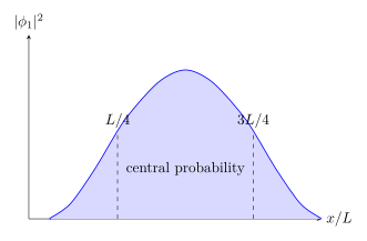
已知: 无限阱基态,求 \(L/4<x<3L/4\) 的概率。
系统与坐标: \(0<x<L\),位置测量在实验室系。
模型: 使用归一化 \(\phi_1=\sqrt{2/L}\sin(\pi x/L)\)。
积分:
\[P=\frac{2}{L}\int_{L/4}^{3L/4}\sin^2\left(\frac{\pi x}{L}\right)dx =\frac12+\frac1\pi =0.818.\]
检查: 区间占总宽一半,但位于基态密度峰附近,故 \(P>0.5\);\(0<P<1\)。
解释: 概率不是由区间长度单独决定,而是由 \(\lvert\phi\rvert^2\) 加权。
Example 3 — 有限阱束缚态计数
已知: 电子有限阱全宽 \(2a=1.00\,\mathrm{nm}\),外部高度 \(V_0=10.0\,\mathrm{eV}\)。
对象与 frame: 对称阱静止系;阱内能量零点为 0。
模型理由: 一维矩形有限阱,恒定电子质量。
计算:
\[z_0=a\frac{\sqrt{2m_eV_0}}{\hbar} =(0.500\,\mathrm{nm})(5.123\,\mathrm{nm^{-1}\,eV^{-1/2}})\sqrt{10.0\,\mathrm{eV}} =8.10.\]
\[N=\left\lceil\frac{2z_0}{\pi}\right\rceil =\lceil5.16\rceil=6.\]
单位与有效数字: \(z_0,N\) 无量纲;\(N\) 必为整数。
阈值检查: \(2z_0/\pi\) 不在整数阈值,故无需边界修正。
解释: 六态按 even、odd、even、odd、even、odd 排列;具体能量仍需解超越方程。
Example 4 — 两能级叠加的位置振荡
已知: 无限阱初态 \(\psi(x,0)=[\phi_1(x)+\phi_2(x)]/\sqrt2\)。
系统与参考系: 静止阱 \(0<x<L\);求 \(\langle x\rangle(t)\)。
模型: Hamiltonian time-independent,系数模方固定,relative phase 演化。
矩阵元:
\[\langle1|x|1\rangle=\langle2|x|2\rangle=\frac L2, \qquad \langle1|x|2\rangle=-\frac{16L}{9\pi^2}.\]
又 \(E_2-E_1=3\pi^2\hbar^2/(2mL^2)\),所以
\[\langle x\rangle(t)=\frac L2- \frac{16L}{9\pi^2} \cos\left(\frac{E_2-E_1}{\hbar}t\right).\]
检查: \(\langle x\rangle\) 在 \(0.320L\) 与 \(0.680L\) 间振荡,始终在阱内;周期为 \(2\pi\hbar/(E_2-E_1)\)。
解释: 每个本征态密度静止,运动来自二者交叉项的相位变化。
Lesson synthesis / 全课综合
束缚态的核心不是“粒子碰墙”,而是三项约束的交集:
- 在每个势能区解定态方程;
- 满足墙或有限跳跃处的边界连续性;
- 在全空间平方可积。
无限墙把相位条件变成 \(kL=n\pi\);有限墙把它变成 even/odd 超越方程。两者都离散化能量。单一本征态只有整体相位,密度不动;多本征态叠加保留不同 \(E_n\) 的 relative phase,于是产生可观测的含时干涉。
Formula-and-decision table / 公式与决策表
| Task | Formula or test | Use condition | Caution |
|---|---|---|---|
| infinite-well state | \(\phi_n=\sqrt{2/L}\sin(n\pi x/L)\) | \(0<x<L\), infinite walls | \(n=1,2,\ldots\) |
| infinite-well energy | \(E_n=n^2\pi^2\hbar^2/(2mL^2)\) | same model | no zero-energy state |
| node count | internal nodes \(=n-1\) | ordered 1D bound spectrum | nodes are not trajectories |
| finite-well even | \(z\tan z=\sqrt{z_0^2-z^2}\) | centered symmetric square well | select branches with positive right side |
| finite-well odd | \(-z\cot z=\sqrt{z_0^2-z^2}\) | same | threshold solution is not normalizable |
| state count | \(N=\lceil2z_0/\pi\rceil\) | \(z_0>0\), exact square-well counting | use ceiling; check energy threshold convention |
| two-state beat | \(\omega_{mn}=(E_m-E_n)/\hbar\) | time-independent Hamiltonian | density needs interference matrix element |
Model boundaries / 模型边界
- Infinite well is an ideal limiting model; finite semiconductor wells have band offsets and effective masses.
- Constant-mass matching uses continuity of \(\phi'\); heterostructures with position-dependent effective mass require a current-conserving modified condition.
- The one-dimensional nondegeneracy theorem assumes regular real potentials and normalizable bound states; higher dimensions can be degenerate.
- \(N=\lceil2z_0/\pi\rceil\) is specific to the symmetric square well convention used here, not a universal counting law for arbitrary \(V(x)\).
- A state at \(E=V_0\) with constant asymptotic amplitude is not square integrable and belongs to the continuum threshold.
- A finite sum of eigenstates is mathematically clean; realistic sharply localized states may require infinitely many high-energy components.
Misconception clinic / 易错诊所
- “无限阱有 \(n=0\) 基态。” \(n=0\) 给零函数,不能归一化。
- “基态能量可为零,因为阱内 \(V=0\)。” 空间限制要求非零曲率与动量展宽,故 \(E_1>0\)。
- “有限阱外概率严格为零。” 错;束缚只要求尾巴可积,波函数在阱外指数衰减。
- “每个图解交点都算束缚态,包括 \(E=V_0\)。” 阈值解的尾巴不衰减,不能归一化。
- “能量本征态中的粒子来回运动,所以密度移动。” 单一本征态密度静止;运动样式来自叠加态 relative phase。
- “\(\lvert c_1\rvert^2+\lvert c_2\rvert^2=1\) 就能忽略交叉项。” 归一化不消除局域密度的干涉项。
Practice and retrieval / 练习与提取
1. 从边界到量子数
由 \(\phi=A\sin kx+B\cos kx\) 和 \(\phi(0)=\phi(L)=0\) 推出允许 \(k\)。
Answer 1
\(\phi(0)=0\) 给 \(B=0\);非零 \(A\) 要求 \(\sin(kL)=0\),所以 \(k_n=n\pi/L\),\(n=1,2,\ldots\)。\(n=0\) 只给零函数。
2. 节点与能量排序
一个无限阱本征态有 4 个内部节点。求 \(n\) 与 \(E/E_1\)。
Answer 2
内部节点数为 \(n-1\),故 \(n=5\);\(E_5/E_1=5^2=25\)。
3. 宽度缩放
阱宽减半,固定 \(n\) 的能量如何改变?
Answer 3
\(E_n\propto L^{-2}\),所以宽度减半使能量增为 4 倍,能级差也整体增为 4 倍。
4. 区间概率
无限阱基态在左半区 \(0<x<L/2\) 的概率是多少?为什么无需积分也可判断?
Answer 4
概率为 \(1/2\)。基态密度关于 \(x=L/2\) 对称,左右半区积分相等,总概率为 1。
5. 尾长与束缚强弱
有限阱态的 \(E\) 向 \(V_0\) 靠近时,\(1/\kappa\) 怎样变化?
Answer 5
\(\kappa=\sqrt{2m(V_0-E)}/\hbar\to0\),所以 \(1/\kappa\to\infty\);波函数更深地伸入阱外,束缚变弱。
6. 宇称匹配
从 even interior \(A\cos kx\) 与 exterior \(Fe^{-\kappa(x-a)}\) 在 \(x=a\) 的匹配推导 even 方程。
Answer 6
连续性给 \(A\cos ka=F\)、导数连续给 \(-Ak\sin ka=-\kappa F\);相除得 \(k\tan ka=\kappa\),即 \(z\tan z=\sqrt{z_0^2-z^2}\)。
7. 束缚态计数
若 \(z_0=3\pi/4\),严格束缚态有几个、宇称如何?
Answer 7
\(2z_0/\pi=1.5\),\(N=\lceil1.5\rceil=2\);最低态 even,第二态 odd。
8. 阈值细节
若 \(z_0=\pi/2\),为什么不能说刚出现两个束缚态?
Answer 8
新 odd 解正处于 \(E=V_0\),\(\kappa=0\),外侧不衰减、不可平方可积;因此严格束缚态仍只有一个。此时 \(N=\lceil1\rceil=1\)。
9. 定态密度
证明单一本征态 \(\psi_n=\phi_ne^{-iE_nt/\hbar}\) 的概率密度与时间无关。
Answer 9
\(\lvert e^{-iE_nt/\hbar}\rvert^2=1\),故 \(\lvert\psi_n(x,t)\rvert^2=\lvert\phi_n(x)\rvert^2\);只有整体相位改变。
10. 拍频
叠加 \(c_1\phi_1+c_3\phi_3\) 的局域密度以什么角频率出现交叉项?能量测量概率会振荡吗?
Answer 10
交叉项角频率为 \(\omega_{31}=(E_3-E_1)/\hbar=8E_1/\hbar\)。能量概率 \(\lvert c_1\rvert^2,\lvert c_3\rvert^2\) 不随时间变。
Exit ticket / 退出检核
- 用一句话分别说明“离散能量”来自哪一组数学条件,“含时密度”又来自什么。
- 给定一幅有限阱波函数图,说明如何从尾长、节点数和关于原点的对称性判断束缚强弱、能级顺序和宇称。
References and source notes / 参考资料与来源说明
以下直接来源于 2026-08-29 实际打开核验;正文独立重述,所有图由方程重新构造。
- MIT OpenCourseWare, 8.04 Quantum Physics I, Lecture Notes 11: Infinite and Finite Wells.
- MIT OpenCourseWare, 8.04 Quantum Physics I, Lecture Notes 12: General Properties of Bound States.
- MIT OpenCourseWare, 8.04 Quantum Physics I, Lecture Notes 13: Node Theorem and Oscillator Introduction.
- OpenStax, University Physics Volume 3, 7.4 The Quantum Particle in a Box.
- David Tong, University of Cambridge, Quantum Mechanics, Section 2: One-Dimensional Potentials.
Source-to-content map / 来源—内容映射
| Source | Used for | Knowledge ID / Section | Model boundary or convention |
|---|---|---|---|
| MIT 8.04 Notes 11 | infinite well, finite-well matching and parity | K01–K04 | centered finite square well |
| MIT 8.04 Notes 12 | bound-state normalizability and one-dimensional structure | K03–K04 | real one-dimensional potentials |
| MIT 8.04 Notes 13 | nodes and ordered bound spectrum | K02, K04 | node theorem context |
| OpenStax 7.4 | box normalization, energies and probabilities | K01–K02 | infinite-wall pedagogical model |
| Tong Section 2 | finite-well transcendental equations and bound states | K03–K05 | stationary states and parity |
复习与拓展
- 下一课用光滑二次势替代方墙,并用 ladder operators 直接产生整套离散谱。
- States, Bases, and Operators 将把 \(\{\phi_n\}\) 解释为 Hilbert-space orthonormal basis,并统一离散展开与连续表象。
- 双阱和周期势会把本课的单阱能级通过 tunneling 变成劈裂或能带,是固体量子理论的入口。