
Learning objectives / 学习目标
完成本课后,你应能:
- 从 \(\hat H=\hat H_0+\lambda\hat V\) 推导非简并能量至二阶、态至一阶,并识别小分母。
- 在简并子空间内构造并对角化 \(W_{ab}=\langle a\rvert\hat V\lvert b\rangle\),解释 good basis 与能级劈裂。
- 用 Rayleigh quotient 证明基态变分上界,选择含物理尺度的 trial state 并优化参数。
- 由局域动量 \(p(x)\) 写出 WKB 允许区、禁阻区解,使用 turning-point connection formula 与量子化条件。
- 对每种近似检查量纲、极限、小参数及边界条件,而不是只套公式。
Prerequisites / 先修知识
- States, Bases, and Operators:本征基、矩阵元与完备性。
- Quantum Harmonic Oscillator:梯算符与奇偶性。
- Hydrogen Atom:简并谱、径向尺度与可解基准。
- 数学:Hermitian matrix diagonalization、Taylor series、Gaussian integral 与常微分方程渐近思想。
Scope and conventions / 范围与约定
- 研究孤立、非相对论系统的定态 Schrödinger 问题;\(\lambda\) 是 bookkeeping parameter,最后通常取 \(1\)。
- \(\hat H_0\lvert n^{(0)}\rangle=E_n^{(0)}\lvert n^{(0)}\rangle\),基矢正交归一;采用 intermediate normalization \(\langle n^{(0)}\vert n\rangle=1\)。
- WKB 只在一维 smooth potential 和 simple turning point 附近讨论;允许区用 \(p(x)=\sqrt{2m[E-V(x)]}\) 与 \(k(x)=p(x)/\hbar\),禁阻区用 \(\kappa(x)=\sqrt{2m[V(x)-E]}/\hbar\)。
- SI 为默认单位;能量也可用 eV。trial state 必须属于 Hamiltonian 的定义域并满足必要边界条件。
- 本课不覆盖多参数 resummation、path-integral semiclassics、instanton 或数值微扰自动化。
Notation and modeling contract / 符号与建模契约
| Symbol | Meaning | Unit |
|---|---|---|
| \(\lambda\) | 无量纲微扰标记参数 | 1 |
| \(\hat V\) | time-independent perturbation | J |
| \(E_n^{(r)},\lvert n^{(r)}\rangle\) | \(\lambda^r\) 阶修正 | J,1 |
| \(\Delta_{nm}=E_n^{(0)}-E_m^{(0)}\) | 未扰能级差 | J |
| \(W=P\hat VP\) | 简并子空间中的有效微扰 | J |
| \(\mathcal E[\phi]\) | Rayleigh quotient | J |
| \(p(x)\) | 允许区 classical local momentum | \(\mathrm{kg\,m\,s^{-1}}\) |
| \(k(x)=p(x)/\hbar\) | 允许区 local wave number | \(\mathrm{m^{-1}}\) |
| \(\kappa(x)\) | 禁阻区 inverse decay length | \(\mathrm{m^{-1}}\) |
1. Nondegenerate perturbation theory / 非简并微扰论
Knowledge ID: P07-U07-L01-K01
设目标未扰能级 \(E_n^{(0)}\) 非简并,展开
\[E_n=E_n^{(0)}+\lambda E_n^{(1)}+\lambda^2E_n^{(2)}+\cdots,\]
\[\lvert n\rangle=\lvert n^{(0)}\rangle+\lambda\lvert n^{(1)}\rangle+\cdots.\]
逐阶代入 eigenvalue equation,左乘 \(\langle n^{(0)}\rvert\) 得
\[E_n^{(1)}=V_{nn}, \qquad E_n^{(2)}=\sum_{m\ne n}\frac{\lvert V_{mn}\rvert^2}{E_n^{(0)}-E_m^{(0)}}.\]
态修正为
\[\lvert n^{(1)}\rangle=\sum_{m\ne n}\frac{V_{mn}}{E_n^{(0)}-E_m^{(0)}}\lvert m^{(0)}\rangle.\]
对基态,所有分母为负,因此 \(E_0^{(2)}\le0\)。这与 exact ground state energy 允许通过 mixing 降低相符。若某个 \(\Delta_{nm}\) 太小,展开参数不再小,应把近简并态共同纳入有效子空间。
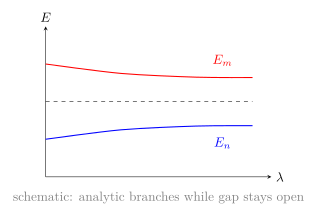
图 1 强调 nondegenerate expansion 所追踪的是一条与 \(\lambda=0\) 连续相连、且与其他能级保持间隔的 branch。
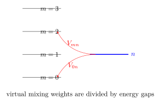
图 2 把二阶和式画成经由所有其他未扰态的 virtual mixing;箭头不是真实含时跃迁。
2. Degenerate perturbation theory / 简并微扰论
Knowledge ID: P07-U07-L01-K02
若 \(d\) 个态共享 \(E_D^{(0)}\),先定义 projector \(P\) 到该子空间,并求
\[W_{ab}=\langle a\rvert\hat V\lvert b\rangle, \qquad a,b=1,\ldots,d.\]
\(W\) 的 eigenvectors 是 zeroth-order good states,eigenvalues \(w_\alpha\) 是一阶能量修正。若 \(W\) 仍有简并,需利用 symmetry 或更高阶 effective Hamiltonian。直接把任意旧 basis 代入 \(V_{aa}\) 会产生 basis-dependent “答案”,因而不物理。
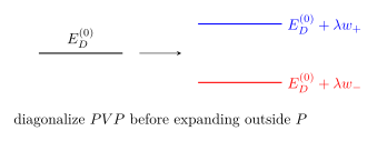
图 3 显示一阶劈裂;其重心和间距由 \(\operatorname{tr}W\) 与 eigenvalue difference 决定。
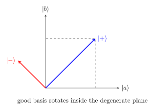
图 4 将 good basis 表示为简并平面内的旋转;完整 Hilbert space 并未缩成二维,只是先处理最危险的小分母。
3. Variational principle / 变分原理
Knowledge ID: P07-U07-L01-K03
对归一化 trial state \(\lvert\phi\rangle=\sum_nc_n\lvert n\rangle\),
\[\mathcal E[\phi]=\frac{\langle\phi\rvert\hat H\lvert\phi\rangle}{\langle\phi\vert\phi\rangle} =\frac{\sum_n\lvert c_n\rvert^2E_n}{\sum_n\lvert c_n\rvert^2}\ge E_0.\]
因此优化得到的是 ground-state energy 的上界,不是任意 excited-state 的自动上界。trial family 应编码 boundary condition、symmetry、node 和 characteristic length。参数越多,上界不会变差,但 over-parameterization 会使数值优化病态。
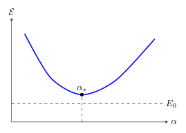
图 5 表示 trial family 的 energy landscape:minimum 仍在 exact \(E_0\) 之上;若算出更低值,通常是积分或 domain 错误。
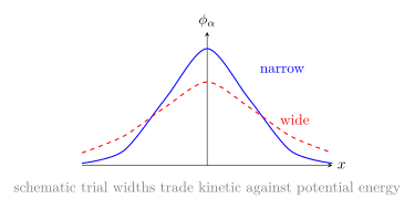
图 6 说明 localization 会增大 kinetic energy,而过宽会提高 confining potential energy,最佳宽度由竞争决定。
4. WKB approximation and connection formulas / WKB 近似与连接公式
Knowledge ID: P07-U07-L01-K04
在允许区 \(E>V\),统一用 local wave number \(k(x)=p(x)/\hbar\),leading WKB form 是
\[\psi(x)\approx\frac{1}{\sqrt{k(x)}} \left[Ae^{i\int^xk(x')dx'}+Be^{-i\int^xk(x')dx'}\right].\]
在禁阻区 \(V>E\),取一个 simple turning point \(x_t\),并先约定允许区在 \(x<x_t\)、禁阻区在 \(x>x_t\):
\[\psi(x)\approx\frac{1}{\sqrt{\kappa(x)}} \left[C_{\mathrm{g}}e^{\int_{x_t}^x\kappa(x')dx'}+C_{\mathrm{d}}e^{-\int_{x_t}^x\kappa(x')dx'}\right].\]
局域条件可写为 \(\lvert k'/k^2\rvert\ll1\)(等价于 \(\lvert\hbar p'/p^2\rvert\ll1\))。它在 turning point 必然失败,必须用 Airy local solution 匹配。对上述朝向,禁阻区的 decaying branch 与允许区的完整 coefficient/phase connection pair 是
\[\frac{C}{\sqrt{\kappa(x)}} e^{-\int_{x_t}^{x}\kappa(x')dx'} \longleftrightarrow \frac{2C}{\sqrt{k(x)}} \cos\left(\int_x^{x_t}k(x')dx'-\frac{\pi}{4}\right).\]
若允许区和禁阻区朝向互换,积分上下限也要随之互换;不能只搬用相位而忽略 coefficient 2。把两个 simple turning points \(x_1,x_2\) 的 decaying 外侧解分别连接到中间允许区,可得 bound-state quantization:
\[\int_{x_1}^{x_2}p(x)dx=\left(n+\frac12\right)\pi\hbar.\]
隧穿 leading exponent 为
\[T\sim\exp\left[-2\int_{x_1}^{x_2}\kappa(x)dx\right],\]
但 pre-exponential factor 依赖 barrier shape 与 matching,不能由指数近似精确给出。
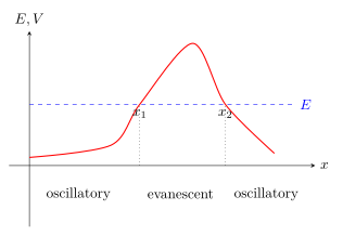
图 7 把 two turning points 与三类区域对齐;实线势能与虚线能量的交点才是 turning points。
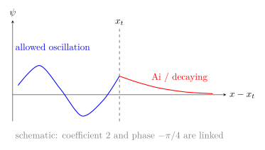
图 8 画的是与 Airy-\(\mathrm{Ai}\) 对应的 decaying branch:离开 \(x_t\) 进入禁阻区后振幅下降;它与左侧振荡解的 coefficient 2 和 phase \(-\pi/4\) 必须作为同一 connection pair 使用。
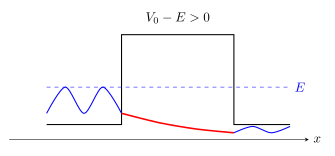
图 9 显示 rectangular barrier 的 incident、evanescent 与 transmitted amplitudes;实际 reflection wave 未单独绘出,故标为 schematic。
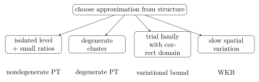
图 10 是方法选择树:先识别控制参数与谱结构,再计算,而不是按题目关键词机械选公式。
Worked Examples / 完整例题
Worked Example 1 — 两能级的二阶能移
已知。 \(H_0=\operatorname{diag}(0,\Delta)\),\(\Delta=2.00\,\mathrm{eV}\),\(V_{12}=V_{21}=0.100\,\mathrm{eV}\),对角元为零,\(\lambda=1\)。
系统、参考系与模型。 孤立两态系统;能量零点取低态。因 \(\lvert V_{12}/\Delta\rvert=0.0500\ll1\),用 nondegenerate PT。
方程与计算。 \(E_1^{(1)}=0\),\(E_1^{(2)}=-\lvert V_{21}\rvert^2/\Delta=-0.00500\,\mathrm{eV}\)。exact lower eigenvalue 是 \([\Delta-\sqrt{\Delta^2+4V^2}]/2=-0.00499\,\mathrm{eV}\)。
检查与解释。 单位为 eV;基态二阶修正应为负。误差约 \(10^{-5}\,\mathrm{eV}\),与下一非零阶约 \((V/\Delta)^4\Delta\) 的量级一致。
Worked Example 2 — 二重简并的 good basis
已知。 在 \(\{\lvert a\rangle,\lvert b\rangle\}\) 中 \(W=\begin{pmatrix}0.30&0.20\\0.20&0.30\end{pmatrix}\,\mathrm{eV}\)。
系统与模型。 只先处理能量 \(E_D\) 的二重简并空间;与外部态的 gap 足够大。
方程与计算。 eigenvectors 是 \(\lvert\pm\rangle=(\lvert a\rangle\pm\lvert b\rangle)/\sqrt2\),eigenvalues \(w_+=0.50\,\mathrm{eV}\)、\(w_-=0.10\,\mathrm{eV}\)。故一阶能量为 \(E_D+0.50\lambda\,\mathrm{eV}\) 与 \(E_D+0.10\lambda\,\mathrm{eV}\)。
检查与解释。 trace \(0.60\,\mathrm{eV}\)、determinant \(0.05\,\mathrm{eV^2}\) 与 eigenvalues 一致;在旧 basis 中只读 \(0.30\,\mathrm{eV}\) 会错过 \(0.40\,\mathrm{eV}\) 的劈裂。
Worked Example 3 — Gaussian 变分宽度
已知。 一维 harmonic oscillator,trial \(\phi_a=(\pi a^2)^{-1/4}e^{-x^2/(2a^2)}\)。
系统、坐标与模型。 孤立粒子,\(x=0\) 为势阱中心,\(H=p^2/(2m)+m\omega^2x^2/2\);trial 满足归一化与无穷远边界。
方程。 \(\langle p^2\rangle=\hbar^2/(2a^2)\)、\(\langle x^2\rangle=a^2/2\),所以 \(\mathcal E(a)=\hbar^2/(4ma^2)+m\omega^2a^2/4\)。令导数为零得 \(a_*=\sqrt{\hbar/(m\omega)}\),\(\mathcal E(a_*)=\hbar\omega/2\)。
检查与解释。 两项单位均为 J;\(a\to0\) 时 kinetic divergence,\(a\to\infty\) 时 potential divergence,故驻点是全局 minimum。trial family 恰含 exact ground state,所以上界取等号。
Worked Example 4 — 电子穿越矩形势垒
已知。 电子遇到宽 \(a=0.500\,\mathrm{nm}\) 的势垒,\(V_0-E=4.00\,\mathrm{eV}\)。
系统、坐标与模型。 势垒沿 \(x\),入射从左向右;使用 leading WKB,忽略 prefactor。
计算。 \(\kappa=\sqrt{2m_e(V_0-E)}/\hbar=10.25\,\mathrm{nm^{-1}}\),故 \(2\kappa a=10.25\),\(T\sim e^{-10.25}=3.54\times10^{-5}\)。
检查与解释。 指数无量纲;增大 \(a\) 或 \(V_0-E\) 会单调减小 \(T\)。矩形势垒边缘不是 smooth turning point,因此这个数只给 exponential scale,精确 prefactor 应由分段 matching 得到。
Lesson synthesis / 全课综合
一条可靠流程是:先选可解 \(H_0\) 与控制参数;再检查目标能级是否隔离;简并则先对角化 \(PVP\);没有自然小参数时尝试 variational upper bound;空间相位缓变且目标是高量子数或 tunneling exponent 时用 WKB;最后以 exact limit、量纲、symmetry 与误差尺度交叉检查。
Formula-and-decision table / 公式与决策表
| Need | Formula | Use when | Main limitation |
|---|---|---|---|
| 一阶能移 | \(E_n^{(1)}=V_{nn}\) | isolated nondegenerate level | 不能处理 zero gap |
| 二阶能移 | \(E_n^{(2)}=\sum_{m\ne n}\lvert V_{mn}\rvert^2/\Delta_{nm}\) | coupling-to-gap ratios small | 小分母使级数失效 |
| 简并劈裂 | \(W=PVP\) 的 eigenvalues | exact 或 near-degenerate cluster | 需再估计与 \(Q=1-P\) 的耦合 |
| 基态上界 | \(E_0\le\mathcal E[\phi]\) | trial state 在正确 domain | 不直接给误差下界 |
| WKB validity | \(\lvert\hbar p'/p^2\rvert\ll1\) | smooth potential away from turning points | \(p=0\) 处失效 |
| Decaying WKB connection | \(Ce^{-\int_{x_t}^{x}\kappa dx}/\sqrt{\kappa}\longleftrightarrow2C\cos(\int_x^{x_t}kdx-\pi/4)/\sqrt{k}\) | allowed left, forbidden right, simple turning point | 反向 turning point 要交换积分朝向 |
| WKB quantization | \(\int_{x_1}^{x_2}pdx=(n+1/2)\pi\hbar\) | two simple turning points | hard wall phase 不同 |
| Tunneling exponent | \(T\sim e^{-2\int\kappa dx}\) | thick smooth barrier | prefactor 未必准确 |
Model boundaries / 模型边界
- Perturbation series 常是 asymptotic,不保证对任意 \(\lambda\) 收敛。
- Near-degeneracy 要扩大 model space;把小分母“保留更多小数”不能修复物理。
- Variational principle 的简单上界只针对最低态;excited states 需施加 orthogonality 或使用更一般 min–max theorem。
- Trial state 违反 cusp、parity 或 boundary condition 时,即使积分有限也可能不在 operator domain。
- WKB 需要 action scale \(S\gg\hbar\),在低量子数、尖锐势阶或 turning point 邻域误差可能大。
- Connection phase 取决于 boundary type;hard wall 与 smooth turning point 不可混用同一个 \(1/2\) 修正。
- 隧穿指数忽略 environmental dissipation、many-body channels 与 multidimensional path。
Misconception clinic / 误区诊所
- “微扰势能的数值小即可。” 必须与相关 gap 比较;单位不同或 gap 极小时,绝对值没有判断力。
- “简并态各自取 diagonal expectation。” diagonal element 随 basis 改变;只有 \(PVP\) eigenvalues 是 basis-independent。
- “二阶修正总为负。” 只对 ground state 必为非正;excited state 有上下方中间态,符号可混合。
- “变分能就是 exact energy 的近似,方向未知。” 对合法 trial state,它严格不低于 exact ground energy。
- “参数越多必然更可信。” 上界可下降,但参数相关性与不适当 domain 会掩盖数值病态。
- “WKB 在 turning point 令 \(p=0\) 后仍可代入。” 振幅 \(1/\sqrt p\) 发散,必须用 connection formula。
- “隧穿概率等于衰减振幅。” 概率近似含 exponent 的两倍,并可能有 flux prefactor。
Practice and retrieval / 练习与提取
- K01|概念: 为什么 ground-state \(E_0^{(2)}\) 不会为正?
- K01|计算: 若唯一耦合态高出 \(3.0\,\mathrm{eV}\),矩阵元 \(0.15\,\mathrm{eV}\),求二阶基态修正。
- K01|边界: \(V_{mn}=0.02\,\mathrm{eV}\)、gap \(0.01\,\mathrm{eV}\),能否称为弱微扰?
- K02|矩阵: 求 \(W=\begin{pmatrix}a&b\\b&a\end{pmatrix}\) 的 good states 与 shifts。
- K02|symmetry: 若 \([PVP,\hat Q]=0\),\(\hat Q\) 如何帮助选 good basis?
- K03|证明: 用 spectral expansion 说明 \(\mathcal E[\phi]\ge E_0\)。
- K03|判断: 一个不满足 hard-wall boundary 的 trial function 能否给合法上界?
- K04|量子化: 谐振子 WKB action \(\oint p\,dx=2\pi E/\omega\),求 \(E_n\)。
- K04|趋势: barrier width 加倍,leading \(T\) 如何变化?
- 综合: 某两态 gap 随参数趋零,同时势能空间缓变;说明应先解决什么谱问题,再决定能否用 WKB。
Answers / 答案
- 对 \(m>0\),\(E_0^{(0)}-E_m^{(0)}<0\),而 numerator 非负,故每项非正。
- \(E_0^{(2)}=-(0.15)^2/3.0=-7.5\times10^{-3}\,\mathrm{eV}\)。
- 不能;无量纲 mixing ratio 是 \(2\),级数没有小参数,应把两态共同对角化。
- eigenstates \((\lvert a\rangle\pm\lvert b\rangle)/\sqrt2\),shifts \(a\pm b\)。
- 可在简并空间同时对角化 \(PVP\) 与 \(Q\),以 symmetry labels 分块并减少矩阵维数。
- \(\mathcal E=\sum_nw_nE_n\),其中 \(w_n\ge0\)、\(\sum_nw_n=1\),故它是能量的加权平均,不小于最小值 \(E_0\)。
- 不能;它不在 Hamiltonian 的定义域,integration by parts 与上界证明条件失效。
- \(\oint p\,dx=2\pi(n+1/2)\hbar\),故 \(E_n=(n+1/2)\hbar\omega\)。
- 若原 \(T\sim e^{-2\kappa a}\),加倍后 \(T'\sim e^{-4\kappa a}=T^2\),在同一 prefactor 近似下。
- 先对 near-degenerate subspace 建立有效 Hamiltonian 并对角化,避免小分母;再对所得 adiabatic branch 检查 \(\lvert\hbar p'/p^2\rvert\),不能让 WKB 替代简并处理。
Exit ticket / 离堂检验
- 用“gap ratio、operator domain、turning point”三个词各写一句近似合法性检查。
- 解释为什么 exact diagonalization of \(PVP\) 与 perturbative coupling to \(Q\) 可以同时存在而不矛盾。
References and source notes / 参考资料与来源说明
以下来源均于 2026-08-30 实际打开核验;正文统一采用 SI 与本课符号,所有图依据方程原创绘制。
- MIT OCW 8.06 (2018), Chapter 1: Non-degenerate and Degenerate Perturbation Theory
- MIT OCW 8.06 (2018), Chapter 3: Semiclassical Approximation
- MIT OCW 8.06, Time-Independent Perturbation Theory and WKB video/notes map
- University of Texas at Austin, Upper-Division Quantum Mechanics Notes
- MIT OCW 8.06 (2016), Chapter 1 lecture notes
Source-to-content map
| Source | Used for | Knowledge ID / Section | Model boundary or convention |
|---|---|---|---|
| MIT 8.06 Chapter 1 | nondegenerate and degenerate derivations, validity | K01–K02 | intermediate normalization stated explicitly |
| MIT 8.06 Chapter 3 | WKB local solutions and connection phase | K04 | simple smooth turning points only |
| MIT 8.06 video/notes map | method sequence and worked physical interpretations | K01–K04 | lectures used as direct teaching source |
| UT Austin notes | independent cross-check of perturbation, variational and scattering conventions | K01–K04 | symbols converted to present contract |
| MIT 8.06 (2016) Chapter 1 | perturbation theory and WKB/connection formulae | K01–K02, K04 | variational K03 is instead cross-checked with UT Austin; no source figures copied |
复习与拓展
- 下一课把 expansion parameter 放入 time-evolution operator,得到 transition amplitudes 与 golden rule。
- Scattering 课会把 Born series 视为对 interaction strength 的 perturbation expansion。
- Atomic Physics 将用 degenerate PT 解释 fine、Zeeman 与 Stark splitting。
- 数值扩展可比较 variational upper bound、WKB eigenvalue 与 shooting-method exact value。