
Learning objectives / 学习目标
- 为 ferromagnet、fluid、BEC 等体系选择 order parameter,并识别其在相变中破缺的 symmetry。
- 最小化 Landau free energy,推导 mean-field order parameter、susceptibility 与典型 critical exponents。
- 定义 connected correlation function 与 correlation length,并联系 susceptibility、structure factor 与 critical opalescence。
- 使用 \(\alpha,\beta,\gamma,\delta,\nu,\eta\) 的严格定义,检验 scaling relations 和 universality-class 条件。
- 用 coarse graining、fixed point、relevant/irrelevant variables 解释 universality,而不把 RG flow 当作真实时间演化。
- 判断 mean-field、hyperscaling、thermodynamic limit 与 finite-size scaling 的适用范围。
Prerequisites / 先修知识
- 一级与连续相变、亚稳态和 hysteresis。
- 涨落、thermodynamic limit 与 free energy。
- BEC order parameter 的物理接口。
- 偶函数展开、偏导、极值稳定性、Fourier transform 与 log–log graph。
Scope and conventions / 范围与约定
- 以 equilibrium continuous transition 为主;一级相变用于对照,不详细处理 nucleation dynamics。
- Reduced temperature 定义为 \(t=(T-T_c)/T_c\);\(t>0\) 表示高温侧。外场 \(h\) 与 scalar order parameter \(m\) 共轭,Landau density 含 \(-hm\)。
- 主要示例是 short-range scalar \(\mathbb Z_2\) symmetry(Ising-like)。XY、Heisenberg、gauge、topological 或 quantum critical transitions 不能无条件套用同一指数。
- Critical exponents 描述 thermodynamic-limit asymptotic singularity;finite \(L\)、有限分辨率、重力与杂质会 rounded 或 cut off divergence。
- Mean-field 结果以 superscript MF 或明确文字标注;三维 Ising 数值只作为当前高精度 consensus 的 representative estimates,不宣称由本课推导。
Notation and modeling contract / 符号与建模契约
| Symbol | Meaning | SI unit |
|---|---|---|
| \(m,\phi(\mathbf r)\) | uniform/local order parameter | model-dependent |
| \(h\) | field conjugate to \(m\) | model-dependent |
| \(t\) | reduced temperature \((T-T_c)/T_c\) | 1 |
| \(f_L\) | Landau free-energy density | \(\mathrm{J\,m^{-3}}\) |
| \(G_c(r)\) | connected two-point correlation | model-dependent |
| \(\xi\) | correlation length | m |
| \(\chi\) | susceptibility \(\partial m/\partial h\) | model-dependent |
| \(d\) | spatial dimension | 1 |
| \(a_0\) | Landau quadratic coefficient multiplying reduced temperature \(t\) | model-dependent; \(\mathrm{J\,m^{-3}}\) for dimensionless \(m\) |
| \(b\) | Landau quartic coefficient | model-dependent; \(\mathrm{J\,m^{-3}}\) for dimensionless \(m\) |
| \(c\) | Landau–Ginzburg gradient stiffness | model- and field-normalization-dependent |
| \(\ell\) | coarse-graining length factor, \(\ell>1\) | 1 |
| \(y_t,y_h\) | RG eigenvalues of temperature/field variables | 1 |
Knowledge 1 — Order parameters and broken symmetry / 序参量与对称性破缺
Knowledge ID: P03-U07-L03-K01
1.1 Order parameter 区分 phases,但不是任意“会变化的量”
Order parameter 是在不同 phases 中具有不同 symmetry character 的宏观变量。例如:
- Ising ferromagnet:\(m=M/V\),高温 \(m=0\),低温在 \(h\to0\) 后选 \(m=\pm m_0\)。
- Liquid–gas critical point:\(m\propto\rho-\rho_c\),liquid/vapor exchange 并非严格 microscopic symmetry,但经 field mixing 可落入 Ising universality。
- 在 thermodynamic-limit symmetry-breaking description of an interacting condensate/superfluid 中,complex order parameter \(\psi=\lvert\psi\rvert e^{i\theta}\) 选择 phase \(\theta\),从而破缺 global \(U(1)\) symmetry。Finite number-conserving systems 也可用 off-diagonal long-range order 描述;BEC 与 superfluidity 不自动等价。
在 finite system 且严格 \(h=0\) 时,equilibrium average 可因两 symmetry-related states 互相抵消为零。Spontaneous symmetry breaking 要按顺序取极限:
\[m_{sp}=\lim_{h\to0^+}\lim_{V\to\infty}\langle m\rangle_{V,h}.\]
若交换两个极限,可能得到零。
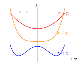
图 1:Landau landscape 从单阱变成对称双阱;低温两个 minima 对应 symmetry-related phases。纵向零点任意。
1.2 外场显式破坏 symmetry 并选择分支
共轭场贡献 \(-hm\)。当 \(h>0\),positive-\(m\) minimum 被降低;这叫 explicit symmetry breaking,不等于 \(h\to0\) 后仍保持非零 \(m\) 的 spontaneous breaking。
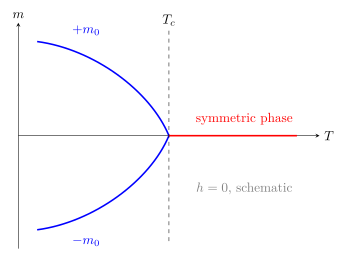
图 2:连续 Ising-like transition 的 order parameter 在 \(T_c\) 连续趋零;曲线没有给出真实 exponent。
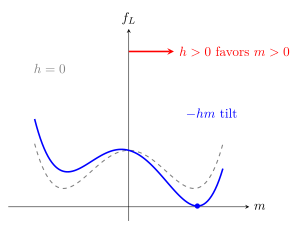
图 3:A conjugate field tilts the double well,选择一个 phase;dashed curve 是未加场基准。
Knowledge 2 — Mean-field models / 平均场模型
Knowledge ID: P03-U07-L03-K02
2.1 Landau expansion 用 symmetry 约束 free energy
对 \(m\to-m\) symmetry,在临界点附近写最低稳定阶:
\[f_L(m)=f_0+\frac{a_0t}{2}m^2+\frac{b}{4}m^4-hm, \qquad a_0>0,\ b>0.\]
Equilibrium 满足
\[\frac{\partial f_L}{\partial m}=a_0tm+bm^3-h=0, \qquad \frac{\partial^2 f_L}{\partial m^2}>0.\]
\(h=0\) 时,
\[m_0= \begin{cases} 0, & t>0,\\ \pm\sqrt{-a_0t/b}, & t<0. \end{cases}\]
所以 mean-field order-parameter exponent 是 \(\beta_{MF}=1/2\)。注意这里的 \(\beta_{MF}\) 是临界指数,不是 inverse temperature。
Worked Example 1 — Landau minima 与 condensation energy
已知: 与全课 reduced-temperature convention 一致,\(f_L-f_0=a_0tm^2/2+bm^4/4\),其中 \(t=(T-T_c)/T_c\)。取 \(a_0=600\ \mathrm{J\,m^{-3}}\)、\(b=8.00\ \mathrm{J\,m^{-3}}\),\(T_c=300\ \mathrm K\)、\(T=294\ \mathrm K\);\(m\) dimensionless。
系统与模型: 均匀 scalar order parameter、\(h=0\)、Landau quartic truncation;忽略 spatial gradients 与 fluctuations。
稳定解: 此处 \(t=(294-300)/300=-0.0200\),quadratic coefficient \(a=a_0t=-12.0\ \mathrm{J\,m^{-3}}\)。
\[m_0=\sqrt{-\frac{a}{b}} =\sqrt{\frac{12.0}{8.00}}=1.225.\]
在 minimum,
\[\Delta f=f_L(m_0)-f_L(0) =-\frac{a^2}{4b} =-4.50\ \mathrm{J\,m^{-3}}.\]
\[\boxed{m_0=\pm1.22,\qquad \Delta f=-4.50\ \mathrm{J\,m^{-3}}.}\]
检查: \(b>0\) 保证大 \(\lvert m\rvert\) 稳定;两 minima 能量相同,符合 \(h=0\) symmetry。数值 \(m_0>1\) 只说明该 dimensionless normalization 不是 bounded spin magnetization;不能在未定义 normalization 时强加 \(\lvert m\rvert\le1\)。
2.2 Susceptibility 与 mean-field exponent set
对 equation of state \(h=a_0tm+bm^3\) 微分,
\[\chi^{-1}=\left(\frac{\partial h}{\partial m}\right)_T =a_0t+3bm^2.\]
高温 \(m=0\) 给 \(\chi\propto t^{-1}\);低温代入 \(m_0^2=-a_0t/b\) 也给 \(\chi\propto\lvert t\rvert^{-1}\),但 amplitude 差二。临界等温线 \(t=0\) 给 \(h=bm^3\)。因此
\[\gamma_{MF}=1, \qquad \delta_{MF}=3, \qquad \alpha_{MF}=0, \qquad \nu_{MF}=\frac12, \qquad \eta_{MF}=0.\]
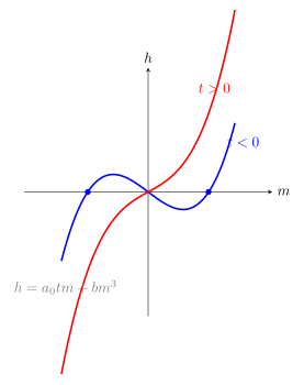
图 4:Mean-field equation of state 在 \(t<0\) 出现多个 stationary branches;稳定性还需检查 curvature。
2.3 Mean field 忽略了空间涨落
Landau–Ginzburg functional 加入 gradient cost:
\[\mathcal F[\phi]=\int \mathrm d^d r\left[ \frac{c}{2}(\nabla\phi)^2+\frac{a_0t}{2}\phi^2 +\frac{b}{4}\phi^4-h\phi \right].\]
Mean field 以 uniform saddle point 取代 fluctuating field。对 short-range scalar theory,\(d_c=4\) 是 upper critical dimension:\(d>4\) 通常有 mean-field exponents;\(d<4\) 的 asymptotic critical region 中 fluctuations 改变指数。\(d=4\) 还会有 logarithmic corrections。
Knowledge 3 — Correlation length and fluctuations / 关联长度与涨落
Knowledge ID: P03-U07-L03-K03
3.1 Connected correlation 排除平均值的平凡乘积
局域 order-parameter field 的 connected correlation 定义为
\[G_c(\mathbf r)= \langle\phi(\mathbf 0)\phi(\mathbf r)\rangle -\langle\phi\rangle^2.\]
临界标度区的统一写法是
\[G_c(r,t)=\frac{1}{r^{d-2+\eta}} \mathcal G_\pm\!\left(\frac{r}{\xi}\right),\]
其中 scaling function \(\mathcal G_\pm(x)\) 在 \(x\gg1\) 时快速(通常指数)衰减,而在 \(x\ll1\) 时趋于有限常数。这样既不把 Gaussian exponential envelope 误写成所有体系的精确 prefactor,也保留临界幂律。
而
\[\boxed{\xi=\xi_\pm\lvert t\rvert^{-\nu}}\]
在 thermodynamic limit 的连续临界点发散。\(\xi_+\) 与 \(\xi_-\) 是非普适 amplitudes;它们的某些 ratios 可普适。
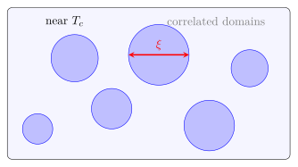
图 5:接近 \(T_c\) 时 correlated fluctuations 跨越越来越大的 \(\xi\);圆形只是示意,不代表 sharp domain boundaries。
3.2 Susceptibility 是 integrated fluctuation
Fluctuation–response relation 在合适 normalization 下把 susceptibility 与 connected correlation 的空间积分联系:
\[\chi\propto\int \mathrm d^d r\,G_c(r).\]
Fourier space 的 Gaussian/Ornstein–Zernike form 为
\[S(q)\propto\frac{1}{q^2+\xi^{-2}}.\]
\(\xi\) 增大使 small-\(q\) scattering 强化;流体的 large density fluctuations 可造成 critical opalescence。恰在 \(t=0\) 且无限体系中,exponential cutoff 消失,
\[G_c(r)\sim r^{-(d-2+\eta)}.\]
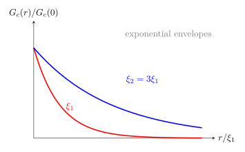
图 6:较大的 correlation length 使 correlations 衰减更慢;图省略 algebraic prefactor 以突出 envelope。
Worked Example 2 — Mean-field 与 3D Ising correlation-length 估计
已知: \(\lvert t\rvert=0.0200\),为教学比较取两模型相同的 \(\xi_0=0.500\ \mathrm{nm}\);mean field 用 \(\nu_{MF}=0.500\),3D Ising representative value 用 \(\nu=0.630\)。求两种 \(\xi\)。
系统与模型: thermodynamic-limit asymptotic power law;人为令 amplitude 相同只为比较 exponent,真实 amplitude 非普适。
计算:
\[\xi_{MF}=0.500(0.0200)^{-0.500}=3.54\ \mathrm{nm},\]
\[\xi_{3D}=0.500(0.0200)^{-0.630}=5.88\ \mathrm{nm}.\]
\[\boxed{\xi_{MF}=3.54\ \mathrm{nm},\qquad \xi_{3D}=5.88\ \mathrm{nm}.}\]
检查: \(\lvert t\rvert\) 无量纲,故单位来自 \(\xi_0\);越接近临界点,两者均增大。不能从这组人为相同 amplitudes 推断真实材料的绝对 \(\xi\) 大小。
Knowledge 4 — Critical exponents and universality / 临界指数与普适性
Knowledge ID: P03-U07-L03-K04
4.1 Exponents 定义 singularity 的形状
在 \(h=0\)、\(t\to0\) 的适当侧,常用定义为
\[C_{sing}\sim\lvert t\rvert^{-\alpha}, \qquad m\sim(-t)^\beta\quad(t<0),\]
\[\chi\sim\lvert t\rvert^{-\gamma}, \qquad \xi\sim\lvert t\rvert^{-\nu},\]
\[m(t=0)\sim\operatorname{sgn}(h)\lvert h\rvert^{1/\delta}, \qquad G_c(r,t=0)\sim r^{-(d-2+\eta)}.\]
Symbol \(\beta\) 在此是 exponent,而 inverse temperature 应写清 \(\beta_T=1/(k_BT)\) 以避免混淆。\(\alpha=0\) 可能对应 finite jump,也可能对应 logarithmic divergence;只写 exponent 不总能区分。
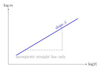
图 7:Power law 在 log–log graph 上给 slope;远离临界区的 crossover 会使数据弯曲。
4.2 Universality class 由少数结构特征决定
不同 microscopic Hamiltonians 可共享 critical exponents。Static universality class 通常取决于:
- spatial dimension \(d\);
- order-parameter components 与 symmetry;
- interaction range;
- quenched disorder、topological constraint 等是否 relevant。
Dynamic critical exponent 还依赖 order parameter 是否 conserved 及其与 hydrodynamic modes 的 coupling;不能只凭 static Ising class 决定 relaxation law。
Short-range 3D Ising representative estimates 为 \(\beta\approx0.3264\)、\(\gamma\approx1.2371\)、\(\nu\approx0.6300\),明显不同于 mean field 的 \(1/2,1,1/2\)。二维 Ising 有 exact \(\beta=1/8\)、\(\gamma=7/4\)、\(\nu=1\)、\(\eta=1/4\),而 \(\alpha=0\) 对应 logarithmic heat-capacity divergence。
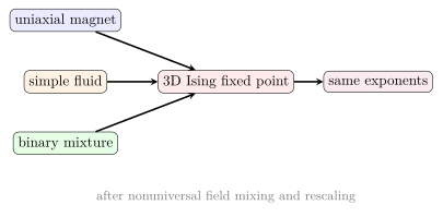
图 8:Microscopically different systems 可流向同一 fixed point;critical amplitudes 本身通常不相同。
4.3 Scaling relations 是一致性检查,不是无条件恒等式
常见 relations 包括
\[\alpha+2\beta+\gamma=2, \qquad \gamma=\beta(\delta-1),\]
\[\gamma=\nu(2-\eta), \qquad 2-\alpha=d\nu.\]
最后一式是 hyperscaling,通常要求 below upper critical dimension 且没有 dangerous irrelevant variable 破坏朴素计数;在 \(d>d_c\) 直接套用会与 mean-field exponents 冲突。
Worked Example 3 — 用 scaling relations 交叉审计 exponent set
已知: 某 3D Ising-like analysis 给 \(\beta=0.326419\)、\(\gamma=1.237075\)。用 Rushbrooke equality 估算 \(\alpha\),再在 hyperscaling 适用的三维情形估算 \(\nu\)。
系统与模型: equilibrium short-range 3D critical point,假设进入 asymptotic scaling regime 且 hyperscaling 有效。
计算:
\[\alpha=2-2\beta-\gamma =2-2(0.326419)-1.237075 =0.110087.\]
\[\nu=\frac{2-\alpha}{d} =\frac{1.889913}{3} =0.629971.\]
\[\boxed{\alpha\approx0.1101,\qquad \nu\approx0.6300.}\]
检查: exponents 无量纲;结果与 3D Ising representative \(\nu\) 一致。此计算不能用于 \(d>4\) 的 naive mean field,因为 hyperscaling assumptions 会失效。
Knowledge 5 — Scaling and renormalization viewpoint / 标度与重整化观点
Knowledge ID: P03-U07-L03-K05
5.1 Scaling hypothesis 把 singular free energy 写成 homogeneous function
令 \(f_s\) 为 free-energy density 的 singular part。Scaling hypothesis 写为
\[\boxed{ f_s(t,h)=\ell^{-d}f_s(t\ell^{y_t},h\ell^{y_h}) }.\]
\(\ell>1\) 是 length rescaling factor,\(y_t=1/\nu\)。选择 \(\ell=\lvert t\rvert^{-1/y_t}\) 可把第一 argument 变为 order one,并导出 power laws 与 exponent relations。
5.2 RG 是“积分掉短尺度,再恢复尺度”的 map
一次 real-space coarse graining:
- 把 linear size \(\ell\) 的 block 内 microscopic variables 合成 block variable;
- integrate out block-internal fluctuations;
- rescale coordinates 和 fields,使 cutoff 恢复原值;
- 得到新的 couplings \(\{K'\}=\mathcal R_\ell(\{K\})\)。
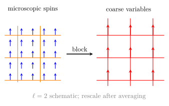
图 9:Block-spin coarse graining 删除短尺度细节并放大长尺度结构;箭头不是时间演化轨迹。
Fixed point \(K^\star\) 满足 \(\mathcal R_\ell(K^\star)=K^\star\)。在其附近,perturbation \(u_i\) 近似按
\[u_i'=\ell^{y_i}u_i\]
变化:\(y_i>0\) relevant、\(y_i<0\) irrelevant、\(y_i=0\) marginal。要到达 critical fixed point,必须 tune relevant temperature-like variable;irrelevant microscopic differences 收缩,正是 universality 的机制。
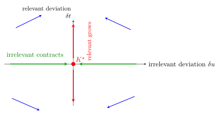
图 10:坐标表示相对 \(K^\star\) 的线性化 deviations;critical surface 上 \(\delta t=0\),irrelevant deviations 收缩到 fixed point,而 relevant deviation 会增长,必须调参归零。
5.3 Finite-size scaling replaces infinity with \(L\)
若无限体系 \(\xi=\xi_0\lvert t\rvert^{-\nu}\),有限 linear size \(L\) 使增长在 \(\xi\sim L\) 时截断。Crossover reduced temperature 约为
\[\lvert t_L\rvert\sim\left(\frac{\xi_0}{L}\right)^{1/\nu}.\]
更一般地 observable \(O\) 可写 \(O(t,L)=L^{-x_O}\mathcal F_O(tL^{1/\nu})\),其中 \(x_O\) 是该 observable 的 RG scaling dimension;例如 magnetization 的 \(x_m=\beta/\nu\)。利用不同 \(L\) 的 data collapse 可估计 \(T_c\) 与 exponents,但 corrections to scaling 和 boundary conditions 必须纳入误差。
Worked Example 4 — 有限样品何时截断 \(\xi\) divergence
已知: \(\xi_0=0.500\ \mathrm{nm}\)、\(\nu=0.630\)、sample size \(L=1.00\ \mathrm{\mu m}\)。估算使 \(\xi\approx L\) 的 \(\lvert t_L\rvert\)。
系统与模型: 单一 correlation length、cubic finite system;忽略 boundary-condition amplitude 与 corrections to scaling。
计算:
\[\lvert t_L\rvert =\left(\frac{0.500\times10^{-9}}{1.00\times10^{-6}}\right)^{1/0.630} =5.76\times10^{-6}.\]
\[\boxed{\lvert t_L\rvert\approx5.8\times10^{-6}.}\]
检查: ratio \(\xi_0/L\) 与 \(t\) 均无量纲;增大 \(L\) 会使 cutoff 更接近 \(t=0\)。这不是温度测量精度本身;若 \(T_c=300\ \mathrm K\),对应温差尺度约 \(1.7\ \mathrm{mK}\),但杂质与温度梯度也可能更早截断。
Lesson synthesis / 全课整合
Order parameter 把 phases 的 symmetry difference 变成可计算变量;Landau theory 用 symmetry 与 stability 给出最小 free-energy model,并能预测 phase structure。临界点附近 correlation length 发散,越来越多 degrees of freedom 共同涨落,恰好破坏了 mean field 的局域平均假设。Scaling 用少数 exponents 描述这种 self-similarity;RG 解释为何 microscopic differences 沿 irrelevant directions 被 coarse graining 消去,而 dimension、symmetry 与 interaction range 决定 fixed point 和 universality class。
建模流程: 选 order parameter 与 conjugate field → 写 symmetry-allowed free energy → 找稳定 extrema → 定义 \(t\)、\(G_c\) 与 \(\xi\) → 判断是否处于 asymptotic/Ginzburg region → 选择 mean-field 或相应 universality class → 检验 exponent relations → 加入 finite-size、disorder 与 dynamic constraints。
Formula-and-decision table / 公式—决策表
| Task | Relation | Use only when | Key caution |
|---|---|---|---|
| spontaneous order | \(m_{sp}=\lim_{h\to0^+}\lim_{V\to\infty}\langle m\rangle\) | equilibrium broken-symmetry phase | order of limits matters |
| Landau free energy | \(f_L=f_0+a_0tm^2/2+bm^4/4-hm\) | scalar \(m\to-m\) symmetry, \(b>0\) | fluctuations omitted |
| mean-field order | \(m_0=\sqrt{-a_0t/b}\) | \(h=0\), \(t<0\) | predicts \(\beta_{MF}=1/2\) only |
| correlation length | \(\xi=\xi_\pm\lvert t\rvert^{-\nu}\) | asymptotic continuous transition | amplitudes are nonuniversal |
| critical correlation | \(G_c(r)\sim r^{-(d-2+\eta)}\) | \(t=0\), thermodynamic limit | finite \(L\) cuts off |
| singular free-energy scaling | \(f_s=\ell^{-d}f_s(t\ell^{y_t},h\ell^{y_h})\) | scaling regime near fixed point | analytic background remains |
| hyperscaling | \(2-\alpha=d\nu\) | below \(d_c\) without dangerous violation | not naive above \(d_c\) |
| finite-size cutoff | \(\lvert t_L\rvert\sim(\xi_0/L)^{1/\nu}\) | one dominant \(\xi\), simple geometry | boundary conditions affect amplitudes |
Model boundaries / 模型边界
- Landau quartic theory assumes an analytic local expansion and appropriate symmetry;cubic invariants、negative quartic coefficient 或 coupling to other fields can drive first-order behavior.
- Mean-field exponents are asymptotically correct above the upper critical dimension for the corresponding short-range model;below it,Ginzburg region requires fluctuation theory.
- Static universality does not determine dynamic universality;conservation laws and hydrodynamic couplings change relaxation exponents.
- Hyperscaling can fail above \(d_c\) or with dangerous irrelevant variables;scaling relations must be tied to derivation assumptions.
- Disorder may be relevant according to the Harris criterion and lead to a different fixed point;sample inhomogeneity can mimic rounded criticality.
- Topological transitions such as BKT need vortex unbinding and essential singularities,not the simple Landau power-law template.
- Quantum critical points add dynamic exponent \(z\) and an imaginary-time dimension;本课主要是 finite-temperature classical criticality。
Misconception clinic / 易错概念诊所
- “任何在相变处变化的量都是 order parameter。” 错;order parameter 要反映 phase/symmetry distinction,heat capacity 通常是 response,不是 order parameter。
- “Finite magnet at \(h=0\) 必定永久选定 \(+m\) 或 \(-m\)。” 不严格;spontaneous breaking 涉及 thermodynamic limit 与极限次序。
- “Landau theory 给出的 \(\beta=1/2\) 是所有连续相变的定律。” 错;它是 mean-field result,三维 fluctuations 通常改写 exponent。
- “Correlation length 是真实 domain 的精确半径。” 错;它是 correlation decay scale,domain 边界未必 sharp。
- “Universality 表示所有物理量都相同。” 错;exponents 与部分 amplitude ratios 可相同,\(T_c\)、absolute amplitudes 与 microscopic spectra 通常不同。
- “RG flow 描述样品随时间走向临界点。” 错;RG parameterizes description under scale change,不是 physical time evolution。
- “看到一段 log–log 直线就证明 critical power law。” 不够;还需控制 background、finite size、corrections to scaling 和可重复的 exponent window。
Practice and retrieval / 练习与检索
1. Choose an order parameter(K01)
分别为 uniaxial ferromagnet 与 liquid–gas critical point 给出合适 scalar order parameter。
Answer
Ferromagnet 可用 magnetization density \(m=M/V\);fluid 可用经适当 field mixing 后的 density difference \(m\propto\rho-\rho_c\)。
2. Limits of symmetry breaking(K01)
为什么定义 \(m_{sp}\) 时先取 \(V\to\infty\) 再取 \(h\to0^+\)?
Answer
有限体系可在 symmetry-related states 间采样,使严格零场平均抵消;先取 thermodynamic limit 使切换 barrier extensive,再撤去 infinitesimal selecting field 才得到 spontaneous branch。
3. Landau minima(K02)
\(f=a t m^2/2+bm^4/4\),\(a,b>0\)。求 \(t<0\) 的 stationary points 并判断稳定性。
Answer
\(m=0\) 与 \(m=\pm\sqrt{-at/b}\)。二阶导在 \(m=0\) 为 \(at<0\),是不稳定 maximum;在非零解为 \(-2at>0\),是两个稳定 minima。
4. Mean-field critical isotherm(K02)
在 \(t=0\),由 \(h=bm^3\) 求 \(m(h)\) 并读出 \(\delta_{MF}\)。
Answer
\(m=\operatorname{sgn}(h)(\lvert h\rvert/b)^{1/3}\),与 \(m\sim\lvert h\rvert^{1/\delta}\) 比较得 \(\delta_{MF}=3\)。
5. Connected correlation(K03)
为什么 \(G_c(r)\) 要减去 \(\langle\phi\rangle^2\)?
Answer
这样排除仅由非零平均序导致的平凡 long-range product,保留真正的 correlated fluctuations;否则 ordered phase 中 \(G\) 即使无涨落也不趋零。
6. Critical opalescence(K03)
用 \(\xi\) 与 \(S(q)\) 解释流体临界乳光。
Answer
临界附近 \(\xi\) 增大,\(S(q)\propto1/(q^2+\xi^{-2})\) 在 small \(q\) 强化;大尺度 density fluctuations 强烈散射可见光,样品呈乳白。
7. Exponent definition(K04)
若 \(m\) 在 \(t<0\) 满足 \(m=A(-t)^{0.326}\),log–log 图斜率是多少?Amplitude \(A\) 是否普适?
Answer
斜率是 \(\beta=0.326\)。Absolute amplitude \(A\) 通常不普适,依单位、normalization 与 microscopic material;特定 amplitude ratios 才可能普适。
8. Widom relation(K04)
给 \(\beta=0.326\)、\(\gamma=1.237\),用 \(\gamma=\beta(\delta-1)\) 估算 \(\delta\)。
Answer
\(\delta=1+\gamma/\beta=1+1.237/0.326\approx4.79\),接近 3D Ising representative value。
9. RG classification(K05)
一次 coarse graining 后 \(u'=\ell^{-1}u\)、\(v'=\ell^{1.5}v\),\(\ell>1\)。判断两变量类型。
Answer
\(u\) 的 eigenvalue exponent \(-1<0\),是 irrelevant;\(v\) 的 \(1.5>0\),是 relevant,必须 tune 才能停在 critical fixed point。
10. Finite-size effect(K03–K05)
为什么 finite system 中 susceptibility peak 有限且峰位可偏离 infinite-system \(T_c\)?
Answer
\(\xi\) 最多增长到 order \(L\),divergence 被 cutoff;scaling variable 是 \(tL^{1/\nu}\),peak rounding 和 pseudocritical shift 都随 \(L\) 改变,并受 boundary conditions/corrections 影响。
Exit ticket / 课末检验
- 从 \(f_L=f_0+a_0tm^2/2+bm^4/4-hm\) 推导 \(m_0\)、\(\chi\) 与 mean-field \(\beta,\gamma,\delta\),再指出一条该推导在 3D 失效的物理原因。
- 用“diverging \(\xi\) → self-similarity → coarse graining → fixed point → relevant/irrelevant variables”五步解释 universality,并加入 finite-size cutoff。
References and source notes / 参考资料与来源说明
- MIT OCW 8.334 Statistical Mechanics II — Lecture Notes 2–8 — Landau–Ginzburg、broken symmetry、correlations、Ginzburg criterion、scaling 与 RG。
- University of Oxford, John Chalker — Theoretical Physics Lecture Notes, Chapter 9 — phase transitions、order parameters、correlation length、critical exponents 与 mean-field limitations。
- NIST, Sengers and Anisimov — Critical Region — fluid criticality、Ising-like asymptotic behavior、mean-field crossover 与 universality。
- Pelissetto and Vicari, Critical Phenomena and Renormalization-Group Theory — O(\(N\)) universality classes、high-precision exponents、equation of state、correlation functions 与 crossover review。
- University of Oxford, John Cardy — Renormalisation Group and Critical Phenomena — RG conceptual basis、scaling、fixed points、low-dimensional and crossover boundaries。
以上链接均于 2026-08-25 实际打开并核对到具体课程、PDF、官方 publication page 或 review。正文把 graduate-level RG 压缩到 Catalog 指定的 UG2→EXT 层级;全部图依据本文模型原创。
Source-to-content map
| Source | Used for | Knowledge ID / Section | Model boundary or convention |
|---|---|---|---|
| MIT 8.334 Notes 2–8 | Landau, correlations, Ginzburg, scaling, RG | K01–K05 | scalar short-range field theory baseline |
| Oxford Chalker Ch. 9 | order parameters and critical phenomenology | K01–K04 | equilibrium thermal transitions |
| NIST Critical Region | fluids, Ising crossover, universality | K03, K04 | asymptotic versus mean-field critical region |
| Pelissetto–Vicari review | 2D/3D exponent estimates and universality | K04, K05 | equilibrium O(\(N\)) short-range classes |
| Oxford Cardy RG course | fixed points, relevant variables, scaling | K05 | conceptual and field-theoretic RG boundary |
复习与拓展
- 下一课进入 transport:critical slowing down 与 dynamic universality 将要求把 equilibrium free energy 与 conservation laws/kinetics 结合。
- Condensed-matter physics 将扩展到 XY/Heisenberg order、Goldstone modes、superconductivity 与 topological transitions。
- Quantum statistical mechanics 将把 \(d\) 维 quantum critical point 映射到含 imaginary time 的 effective classical theory,并引入 dynamic exponent \(z\)。
- Computational physics 将用 Monte Carlo、Binder cumulant 与 finite-size data collapse 提取 universality class。