
Learning objectives / 学习目标
你将能够:
- 用有向截面定义瞬时与平均电流,并从 \(Q(t)\) 图像读取符号和斜率。
- 区分 conventional current 与电子、离子、空穴等真实载流子的运动。
- 使用 \(I=\int\mathbf J\cdot d\mathbf A\) 与 continuity equation 分析局部电荷积累。
- 推导 \(\mathbf J=\sum_sn_sq_s\mathbf v_{d,s}\),并用 Drude 模型连接漂移、碰撞与导电率。
- 把 emf 定义为电源对单位电荷提供的能量,区分 emf、端电压、力与电场。
Prerequisites / 先修知识
- 电荷守恒、electric field 与 potential difference。
- Local Form of Electrostatics:散度、任意控制体积与局部守恒语言。
- 有向面积积分、导数与基本粒子数密度。
Scope, conventions, and notation
- SI 制;\(1\ \mathrm A=1\ \mathrm{C/s}\)。现行 SI 通过精确基本电荷 \(e=1.602\,176\,634\times10^{-19}\ \mathrm C\) 定义 ampere。
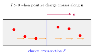
- 对截面 \(S\) 选择法向 \(\hat{\mathbf n}\);沿该法向的 conventional current 为正。
- \(I\) 是针对指定截面的带符号标量;\(\mathbf J\) 是局部矢量场。
- 本课采用准静态 lumped-circuit 直觉,但明确区分缓慢漂移载流子与快速传播的电磁信号。
- 电阻、Joule heating、内阻与完整 circuit rules 留到后续 Lesson。
| Symbol | Meaning | SI unit |
|---|---|---|
| \(I\) | electric current / 电流 | A |
| \(Q\) | signed charge crossing chosen section | C |
| \(\mathbf J\) | current density / 电流密度 | \(\mathrm{A/m^2}\) |
| \(n_s\) | number density of carrier species \(s\) | \(\mathrm{m^{-3}}\) |
| \(q_s\) | signed carrier charge | C |
| \(\mathbf v_{d,s}\) | drift velocity | \(\mathrm{m/s}\) |
| \(\mathcal E\) | electromotive force / 电动势 | V = J/C |
Knowledge 1 — Current as charge-flow rate / 电流是电荷流率
Knowledge ID: P04-U05-L01-K01
1.1 Instantaneous and average current
固定一个有向截面,令 \(Q_+(t)\) 表示从参考时刻起沿正法向净穿过的电荷,则
\[\boxed{I(t)=\frac{dQ_+}{dt}}, \qquad \boxed{I_{\rm avg}=\frac{\Delta Q_+}{\Delta t}}.\]
若正电荷沿 \(-\hat{\mathbf n}\) 运动,或负电荷沿 \(+\hat{\mathbf n}\) 运动,均给负电流。对一维导线,选择参考方向后可用正负号编码方向;“电流大小”是 \(\lvert I\rvert\)。
1.2 Current is a rate, not an inventory
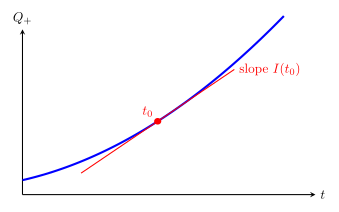
\(I\) 不等于导线内“现有多少电荷”。稳定电流中每一小段近似不积累净电荷,但电荷持续穿过截面。若
\[Q_+(t)=Q_0+at+bt^2,\]
则 \(I(t)=a+2bt\),即 \(Q\)–\(t\) 曲线的切线斜率。
Worked Example 1 — Reading a time-dependent current
沿选定正方向累计电荷为
\[Q_+(t)=(0.500\ \mathrm C)+(2.00\ \mathrm{C/s})t-(0.300\ \mathrm{C/s^2})t^2.\]
求 \(t=2.00\ \mathrm s\) 的瞬时电流及 \(0\) 到 \(2.00\ \mathrm s\) 的平均电流。
- 截面与正方向: 题中 \(Q_+\) 已按选定法向计号。
- 模型: 连续可微的宏观电荷流率。
- 计算:
\[I(t)=2.00-0.600t, \qquad I(2.00)=\boxed{0.800\ \mathrm A}.\]
\[I_{\rm avg}=\frac{Q_+(2)-Q_+(0)}{2.00} =\frac{3.30-0.500}{2.00} =\boxed{1.40\ \mathrm A}.\]
- 检查: 电流从 \(2.00\ \mathrm A\) 线性降至 \(0.800\ \mathrm A\),区间平均值应等于两端均值 \((2.00+0.800)/2=1.40\ \mathrm A\);\(dQ/dt\) 单位为 C/s = A。
Knowledge 2 — Conventional current and carrier motion / 传统电流方向与载流子运动
Knowledge ID: P04-U05-L01-K02
2.1 Signed charge transport
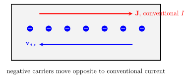
传统电流方向定义为正电荷净运动方向。单一种类载流子时
\[\mathbf J=nq\mathbf v_d.\]
金属中 \(q=-e\),故电子漂移 \(\mathbf v_d\) 与 \(\mathbf J\) 相反;正离子或空穴的漂移与 \(\mathbf J\) 同向。
2.2 Multiple carrier species
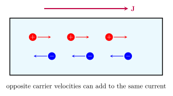
电解质、半导体与等离子体可同时有多种载流子:
\[\boxed{\mathbf J=\sum_sn_sq_s\mathbf v_{d,s}}.\]
负离子向左时 \(q_s<0\) 且 \(v_{d,s}<0\),乘积为正,因而也可与向右的正离子共同贡献向右电流。
Worked Example 2 — Ionic solution with two carriers
在电解质中,\(n_+=2.0\times10^{25}\ \mathrm{m^{-3}}\) 的一价正离子以 \(+1.0\times10^{-5}\ \mathrm{m/s}\) 漂移;同密度负离子以 \(-1.5\times10^{-5}\ \mathrm{m/s}\) 漂移。截面积 \(A=1.00\ \mathrm{cm^2}\)。
- 参考方向: \(+x\);正负离子电荷分别 \(+e,-e\)。
- 模型: 截面上密度与漂移均匀,两种载流子贡献相加。
- 计算:
\[J_x=n_+e v_+ + n_-(-e)v_- =n e(1.0+1.5)\times10^{-5} =80.1\ \mathrm{A/m^2}.\]
\[I=J_xA=(80.1)(1.00\times10^{-4}) =\boxed{8.01\ \mathrm{mA}}.\]
- 检查: 两项均为正;若把所有漂移速度反向,电流也反向;有效数字三位。
Knowledge 3 — Current density and continuity equation / 电流密度与连续性方程
Knowledge ID: P04-U05-L01-K03
3.1 From local flow to total current
对有向截面
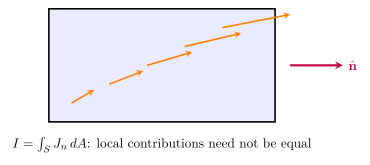
\[\boxed{I=\int_S\mathbf J\cdot d\mathbf A}.\]
只有 \(\mathbf J\) 均匀且垂直截面时才简化为 \(I=JA\)。若载流方向斜穿或截面上不均匀,必须积分法向分量。
3.2 Integral charge balance
对固定控制体积 \(V\),内部电荷
\[Q_V=\int_V\rho\,dV.\]
外向电流为 \(\oint_{\partial V}\mathbf J\cdot d\mathbf A\)。电荷守恒要求
\[\boxed{ \frac{d}{dt}\int_V\rho\,dV =-\oint_{\partial V}\mathbf J\cdot d\mathbf A }.\]
散度定理和 \(V\) 任意给出局部 continuity equation:
\[\boxed{\frac{\partial\rho}{\partial t}+\nabla\cdot\mathbf J=0}.\]
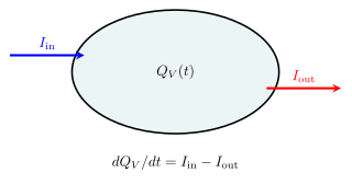
稳恒电流(steady current)时 \(\partial\rho/\partial t=0\),故 \(\nabla\cdot\mathbf J=0\)。这不是说 \(\rho=0\),而是每个小体积没有净积累。
Worked Example 3 — Charge accumulation at a junction
一个小接头视作控制体积。左侧有 \(I_{\rm in}=3.20\ \mathrm A\) 流入,右侧只有 \(I_{\rm out}=2.70\ \mathrm A\) 流出,持续 \(4.00\ \mathrm{ms}\)。
- 系统边界: 包住接头的固定体积;流入取正计入 \(dQ/dt\)。
- 守恒方程:
\[\frac{dQ_V}{dt}=I_{\rm in}-I_{\rm out}=0.500\ \mathrm A.\]
- 计算:
\[\Delta Q=(0.500)(4.00\times10^{-3}) =\boxed{2.00\times10^{-3}\ \mathrm C}.\]
- 检查: 流入大于流出,积累为正;A·s = C。真实金属中如此大的积累会迅速改变局部场并调整电流,所以长期稳态不允许持续不匹配。
Knowledge 4 — Drift velocity and microscopic conduction / 漂移速度与微观导电
Knowledge ID: P04-U05-L01-K04
4.1 Derive \(\mathbf J=nq\mathbf v_d\)
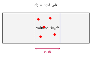
取截面法向为一维正方向,并令带符号标量 \(v_d=\mathbf v_d\cdot\hat{\mathbf n}\)。时间 \(dt\) 内实际穿过截面的载流子数目为 \(nA\lvert v_d\rvert dt\);按所选正方向计号的输运电荷则为 \(dq=nqAv_d\,dt\),可因 \(q\) 或 \(v_d\) 的符号而为负。因此
\[I=nqAv_d, \qquad \boxed{\mathbf J=nq\mathbf v_d}.\]
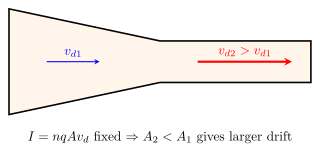
若导线变细且 \(I\)、\(n\) 不变,\(v_d=I/(nqA)\) 增大;这不是单个电子在截面处突然加速后永不碰撞,而是局部 ensemble average 改变。
4.2 Drude model: collisions create finite drift
在最简 Drude 模型中,载流子平均碰撞时间为 \(\tau\)。两次碰撞之间由电场加速,稳态平均漂移
\[\mathbf v_d=\frac{q\tau}{m}\mathbf E.\]
于是
\[\mathbf J=nq\mathbf v_d =\frac{nq^2\tau}{m}\mathbf E =\boxed{\sigma_c\mathbf E}, \qquad \sigma_c=\frac{nq^2\tau}{m}.\]
这里 \(\sigma_c\) 是 conductivity,避免与表面电荷密度 \(\sigma\) 混淆。Drude 是经典平均模型,不能完整描述能带、量子散射或超导。
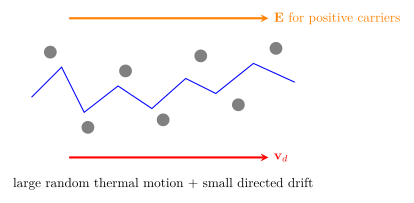
电路信号传播速度由电磁场和介质决定,可接近光速的一定比例;它不等于电子常见的 \(10^{-4}\ \mathrm{m/s}\) 量级漂移速度。
Worked Example 4 — Copper drift, charge throughput, and source energy
一根铜线横截面积 \(A=1.00\ \mathrm{mm^2}\),自由电子密度 \(n=8.50\times10^{28}\ \mathrm{m^{-3}}\),由 \(1.50\ \mathrm V\) 理想电源维持 conventional current \(I=2.00\ \mathrm A\)。求电子漂移速度、\(3.00\ \mathrm s\) 通过截面的电子数,以及电源向这些电荷提供的能量。
- 正方向: conventional current 方向;电子 \(q=-e\),故 \(v_{d,e}<0\)。
- 漂移:
\[v_{d,e}=\frac{I}{nqA} =\frac{2.00}{(8.50\times10^{28})(-e)(1.00\times10^{-6})} =\boxed{-1.47\times10^{-4}\ \mathrm{m/s}}.\]
- 电荷与粒子数:
\[\Delta Q=I\Delta t=6.00\ \mathrm C, \qquad N=\frac{\Delta Q}{e}=\boxed{3.75\times10^{19}}.\]
- 电源能量: 每库仑给 \(1.50\ \mathrm J\),
\[W=\mathcal E\Delta Q=(1.50)(6.00)=\boxed{9.00\ \mathrm J}.\]
- 检查: 电子漂移与 conventional current 反向;巨大粒子数与很小漂移并不矛盾;V·C = J。
Knowledge 5 — Electromotive force and sources / 电动势与电源
Knowledge ID: P04-U05-L01-K05
5.1 A source is an energy pump
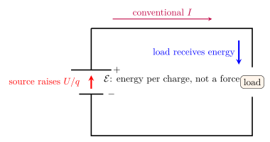
电动势不是机械“力”。它是电源内非静电机制(化学、机械、光等)对单位电荷提供的能量:
\[\boxed{\mathcal E=\frac{dW_{\rm source}}{dq}}, \qquad [\mathcal E]=\mathrm{J/C}=\mathrm V.\]
更一般地,对绕一周的单位电荷,source force per charge \(\mathbf f_{\rm s}\) 的线积分为
\[\boxed{\mathcal E=\oint\mathbf f_{\rm s}\cdot d\boldsymbol\ell}.\]
理想电源把电荷从较低电势端“泵”到较高电势端;外电路中静电场再把电势能传递给负载。开路时理想源端电压等于 emf;有电流的真实源因内阻和极化,端电压可不同,详见下一课。
5.2 Source power at the terminal level
若正电流 \(I\) 通过理想 source 的低势端进入、高势端离开,source 对电荷提供功率
\[\boxed{P_{\rm source}=\mathcal EI}.\]
符号取决于端口约定:若电流进入 source 的高势端,器件吸收能量(充电)。在本课中总应先画电流方向与端极性,再判断供能/吸能。
Lesson synthesis / 全课整合
Formula-and-decision table
| Question | Use | Conditions / warning |
|---|---|---|
| how much charge crosses? | \(I=dQ_+/dt\) | define section orientation |
| local-to-total current | \(I=\int_S\mathbf J\cdot d\mathbf A\) | use normal component |
| carrier model | \(\mathbf J=\sum n_sq_s\mathbf v_{d,s}\) | \(q_s\) and velocity are signed/vector |
| charge accumulation | \(\partial_t\rho+\nabla\cdot\mathbf J=0\) | fixed spatial control volume |
| simple metal response | \(\mathbf J=\sigma_c\mathbf E\) | linear, isotropic, ordinary conductor |
| source energy | \(dW=\mathcal E\,dq\) | emf is not force |
| ideal source power | \(P=\mathcal EI\) | sign from current/terminal convention |
Model boundaries / 模型边界
- \(I\) 的 lumped-circuit 描述要求横截面尺度和传播延迟可忽略;高频分布参数系统需完整 Maxwell 模型。
- Drude 模型是经典平均近似;不精确描述半导体能带、量子霍尔效应、超导或强场非线性。
- \(\mathbf J=\sigma_c\mathbf E\) 只在线性、局域、各向同性近似下成立;一般 \(\mathbf J\) 可有张量和非局域响应。
- 漂移速度不是信号速度,也不是电子热运动的典型速率。
- 理想 source 保持 emf;真实 source 的端电压取决于电流、内阻、温度与化学状态。
Misconception clinic / 易错概念诊所
| Misconception | Correction |
|---|---|
| “电流是矢量。” | 对指定支路/截面它是带符号标量;\(\mathbf J\) 才是矢量。 |
| “电子沿电流方向运动。” | 金属电子带负电,平均漂移与 conventional current 相反。 |
| “两种离子反向移动,电流必抵消。” | 负电荷与负速度乘积为正,可能相加。 |
| “稳定电流意味着电荷不动。” | 意味着局部不积累净电荷;载流子持续漂移。 |
| “灯立刻亮说明电子接近光速。” | 快的是电磁场调整/信号,电子漂移通常很慢。 |
| “emf 是一种力。” | 它是 source 对单位电荷提供的能量,单位是 volt。 |
Practice and retrieval / 练习与检索
- \(5.00\ \mathrm C\) 在 \(2.00\ \mathrm s\) 内沿正方向穿过截面,平均电流是多少?
Answer 1
\(I_{\rm avg}=\Delta Q/\Delta t=2.50\ \mathrm A\)。
- 每秒有 \(3.00\times10^{18}\) 个电子向左穿过截面。若正方向向右,电流是多少?
Answer 2
\(I=(-e)(-3.00\times10^{18}\ \mathrm{s^{-1}})=+0.481\ \mathrm A\),conventional current 向右。
- 为什么 \(I\) 是标量而 \(\mathbf J\) 是矢量?
Answer 3
\(I\) 已经对一个有向截面把局部法向流积分成单一带符号数;\(\mathbf J\) 仍在每点保留流动方向。
- 圆导线半径 \(1.00\ \mathrm{mm}\),均匀 \(J=2.00\times10^5\ \mathrm{A/m^2}\),求 \(I\)。
Answer 4
\(I=J\pi r^2=(2.00\times10^5)\pi(10^{-3})^2=0.628\ \mathrm A\)。
- 固定控制体积净外向电流为 \(-0.200\ \mathrm A\)。内部电荷变化率是多少?
Answer 5
\(dQ_V/dt=-I_{\rm outward}=+0.200\ \mathrm{C/s}\),内部正电荷增加。
- 稳恒电流为何要求 \(\nabla\cdot\mathbf J=0\)?
Answer 6
稳恒意味着 \(\partial\rho/\partial t=0\);代入 continuity equation 即得。
- 相同材料、相同电流的两段导线,第二段面积为第一段一半。漂移速度比是多少?
Answer 7
\(v_d=I/(nqA)\),所以第二段漂移速度大小为第一段 2 倍。
- \(n=1.0\times10^{28}\ \mathrm{m^{-3}}\)、正载流子 \(q=e\)、\(v_d=2.0\times10^{-4}\ \mathrm{m/s}\),求 \(J\)。
Answer 8
\(J=nqv_d=3.20\times10^5\ \mathrm{A/m^2}\),方向同漂移。
- \(9.00\ \mathrm V\) 电源搬运 \(0.250\ \mathrm C\) 电荷,提供多少能量?
Answer 9
\(W=\mathcal E q=(9.00)(0.250)=2.25\ \mathrm J\)。
- 理想 \(12.0\ \mathrm V\) source 以 \(3.00\ \mathrm A\) 向外供电,功率是多少?
Answer 10
\(P=\mathcal EI=36.0\ \mathrm W\);若同方向电流改为进入正端,则 source 吸收功率。
Exit ticket
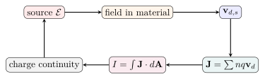
一根金属线接到电池后灯几乎立即亮。用 \(I\)、\(\mathbf J\)、\(\mathbf v_d\)、\(\mathcal E\) 和 continuity equation 写出不超过五句的因果链,并指出哪个速度很慢。
Exit-ticket benchmark
source 以 emf 为单位电荷供能并建立电磁场;场在导体中驱动电子产生小的反向漂移 \(\mathbf v_d\);\(\mathbf J=nq\mathbf v_d\),截面积分给 \(I\);continuity equation 使表面电荷和局部电流迅速自洽而不长期积累;很慢的是载流子的漂移,快速的是电磁信号传播。
References and source notes / 参考资料与来源说明
以下资料均于 2026-08-26 实际访问核验。
- OpenStax University Physics Volume 2, 9.1 Electrical Current
- OpenStax University Physics Volume 2, 9.2 Model of Conduction in Metals
- OpenStax University Physics Volume 2, 10.1 Electromotive Force
- MIT OpenCourseWare 8.022 Lecture 7 — Current and Continuity Equation
- NIST SP 330, Section 2 — The ampere
Source-to-content map
| Source | Used for | Knowledge ID / Section | Model boundary or convention |
|---|---|---|---|
| OpenStax 9.1 | \(I=dQ/dt\), conventional current, complete path | K01, K02 | current direction is positive-charge convention |
| OpenStax 9.2 | current density, drift, signal versus carrier speed | K03, K04 | ordinary metal model |
| OpenStax 10.1 | emf as work per unit charge, ideal source | K05 | open-circuit idealization separated from loaded terminal voltage |
| MIT 8.022 Lecture 7 | continuity equation and current-density cross-check | K01–K04 | fixed control-volume sign convention |
| NIST SP 330 | current SI unit and exact elementary charge | K01, conventions | post-2019 SI definition |
复习与拓展
- Resistance and Electrical Energy 将加入 \(R\)、\(\rho_{\rm resistivity}\)、Joule heating 与内阻,需避免与本课 charge density \(\rho\) 混淆。
- Circuit Analysis 的 junction rule 是 continuity equation 的 lumped 版本。
- Maxwell–Ampère law 将解释时变电场与 displacement current 的更完整守恒结构。