
Learning objectives / 学习目标
完成本课后,你应当能够:
- 区分 Dirichlet、Neumann 与 mixed boundary data,陈述并证明相应 electrostatic uniqueness result。
- 在 Cartesian、cylindrical 和 spherical geometry 中选择分离变量的本征函数,并由边界数据确定系数。
- 定义满足指定边界的 Green function,用 Green identity 构造势,并正确解释 image charges 的适用域与能量因子 \(1/2\)。
- 推导局域源的 electric monopole、dipole、quadrupole 以及 magnetic dipole far field。
- 用 source size / observation distance 估计截断误差,并检查边界、单位、奇点与远场极限。
Prerequisites / 先修知识
- Local Form of Electrostatics:\(\nabla^2V=-\rho/\epsilon_0\)。
- Electrostatic potential、导体等势面、surface charge。
- Green’s identities、Fourier series、Legendre polynomials。
- Biot–Savart Law:磁偶极远场。
- 磁静力学中的局域稳恒电流与磁偶极远场;本课在 K04 最小定义 \(\mathbf A\),规范自由留到下一课。
Scope and conventions / 范围与约定
- 静电势定义 \(\mathbf E=-\nabla V\),满足 \(\nabla^2V=-\rho/\epsilon_0\);无电荷区域为 Laplace equation。
- 边界外法向记 \(\hat{\mathbf n}'\),\(\partial/\partial n'=\hat{\mathbf n}'\cdot\nabla'\)。
- Green function 采用约定 \(\nabla'^2G(\mathbf r,\mathbf r')=-4\pi\delta(\mathbf r-\mathbf r')\);若来源采用 \(-\delta\) 约定,\(4\pi\) 因子会重新分配。
- image charges 只放在被排除的数学区域;它们替代边界条件,不是实际导体内部的电荷。
- multipole expansion 要求观察点到选定原点的距离 \(r\) 大于整个局域源的尺度 \(a\);本课以 \(a/r\) 为小参数。
- 采用 SI;图示均为 schematic / not to scale。
Notation and modeling contract / 符号与建模契约
| Symbol | Meaning | SI unit |
|---|---|---|
| \(\Omega,\partial\Omega\) | solution domain and its boundary | — |
| \(V,\rho\) | electrostatic potential and volume charge density | V, \(\mathrm{C\,m^{-3}}\) |
| \(G(\mathbf r,\mathbf r')\) | Green function with stated boundary condition | \(\mathrm{m^{-1}}\) |
| \(\mathbf A\) | magnetostatic vector potential, \(\mathbf B=\nabla\times\mathbf A\) | \(\mathrm{T\,m}\) |
| \(Q,\mathbf p,Q_{ij}\) | electric monopole, dipole, traceless quadrupole moments | C, \(\mathrm{C\,m}\), \(\mathrm{C\,m^2}\) |
| \(\mathbf m\) | magnetic dipole moment | \(\mathrm{A\,m^2}\) |
| \(a/r\) | source-size to observation-distance ratio | dimensionless |
| \(\hat{\mathbf n}'\) | outward normal of source-domain boundary | dimensionless |
Knowledge 1 — Electrostatic uniqueness and boundary conditions / 静电唯一性与边界条件
Knowledge ID: P04-U11-L01-K01
1.1 Boundary data define the problem
Poisson equation alone does not select a unique physical solution; boundary data are part of the model.
- Dirichlet: 给定 \(V\) 在 \(\partial\Omega\) 上的值。
- Neumann: 给定 \(\partial V/\partial n\);还须满足 compatibility condition,解只确定到加法常数。
- Mixed: 在互不重叠的边界部分给定 \(V\) 或其法向导数。
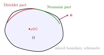
图 1 说明“系统边界”不是可忽略外框;同一 \(\rho\) 配不同边界会产生不同 \(V\)。
1.2 Dirichlet uniqueness proof
设 \(V_1,V_2\) 满足同一 Poisson equation 和同一 Dirichlet data。差函数 \(U=V_1-V_2\) 满足
\[\nabla^2U=0,\qquad U\big|_{\partial\Omega}=0.\]
Green first identity 给
\[\int_\Omega\lvert\nabla U\rvert^2d\tau =\int_{\partial\Omega}U\frac{\partial U}{\partial n}\,da -\int_\Omega U\nabla^2U\,d\tau=0.\]
被积函数非负,所以 \(\nabla U=0\);\(U\) 是常数,而边界值迫使 \(U=0\)。故解唯一。
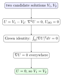
图 2 把唯一性证明压缩为“非负积分为零”;它授权我们用任何满足方程和边界的构造作为物理解。
1.3 Neumann qualification
Neumann data 必须满足由 Poisson equation 导出的 compatibility:
\[\int_{\partial\Omega}\frac{\partial V}{\partial n}\,da =-\frac{1}{\epsilon_0}\int_\Omega\rho\,d\tau.\]
因为只给梯度,\(V+C\) 与 \(V\) 有同一数据,所以最多唯一到加法常数。电场 \(\mathbf E\) 仍唯一。
Knowledge 2 — Separation of variables in common geometries / 常见几何中的分离变量
Knowledge ID: P04-U11-L01-K02
2.1 Product ansatz is a boundary-matched basis
在矩形无源区域,令 \(V(x,y)=X(x)Y(y)\),Laplace equation 给
\[\frac{X''}{X}=-\frac{Y''}{Y}=-k^2.\]
边界决定允许的 \(k\) 与 sin/cos/sinh/cosh 组合;一般边界数据再展开为这些本征函数的级数。
若 \(0<x<a\)、\(0<y<b\),三边接地且
\[V(x,0)=V_0\sin\frac{\pi x}{a},\]
则单一匹配模式是
\[V(x,y)=V_0\sin\frac{\pi x}{a} \frac{\sinh[\pi(b-y)/a]}{\sinh(\pi b/a)}.\]
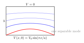
图 3 中红线表示边界势的函数形状,不是物理导线轨迹;蓝线只示意势随 \(y\) 指数型衰减。
2.2 Geometry chooses the eigenfunctions
| Geometry / symmetry | Typical separated functions | Typical boundary coordinate |
|---|---|---|
| Cartesian rectangle | \(\sin kx,\cos kx,\sinh ky,\cosh ky\) | planes |
| Cylindrical | \(e^{im\phi}\) and Bessel/powers | cylinders |
| Spherical, azimuthal symmetry | \(r^\ell,r^{-(\ell+1)},P_\ell(\cos\theta)\) | spheres |
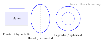
图 4 强调坐标选择由边界几何驱动,而不是由个人偏好驱动。
2.3 Convergence and corners
级数解通常在域内快速收敛,但不连续边界或尖角会产生大梯度与较慢 Fourier convergence。数学理想尖角处场可发散;真实圆角和有限材料尺度会正则化。
Knowledge 3 — Green functions and image methods / 格林函数与镜像法
Knowledge ID: P04-U11-L01-K03
3.1 Green function as boundary-aware point response
定义
\[\nabla'^2G(\mathbf r,\mathbf r')=-4\pi\delta(\mathbf r-\mathbf r').\]
Green second identity 给出
\[V(\mathbf r)=\frac{1}{4\pi\epsilon_0}\int_\Omega \rho(\mathbf r')G(\mathbf r,\mathbf r')\,d\tau' +\frac{1}{4\pi}\int_{\partial\Omega} \left[ G\frac{\partial V}{\partial n'} -V\frac{\partial G}{\partial n'} \right]da'.\]
Dirichlet Green function 在边界上满足 \(G=0\),于是边界项只含已知 \(V\)。Green function 同时编码微分算子、几何和边界条件。
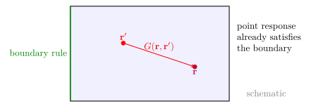
图 5 把 Green function 看成“单位点源的边界适配响应”;对 \(\rho\) 的积分就是响应叠加。
3.2 Grounded-plane image
真实点电荷 \(q\) 位于 \(z=a>0\),无限接地导体占边界 \(z=0\)。在物理域 \(z>0\) 内,可用 \(z=-a\) 处的 image charge \(-q\) 构造
\[V(\rho,z)=\frac{1}{4\pi\epsilon_0} \left[ \frac{q}{\sqrt{\rho^2+(z-a)^2}} -\frac{q}{\sqrt{\rho^2+(z+a)^2}} \right].\]
它在 \(z=0\) 恰为零;由 uniqueness theorem,此构造就是物理域内唯一解。
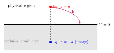
图 6 中蓝色 image 不是真实导体内电荷;它只在 \(z>0\) 复现正确边界势。紫色电场线从正电荷出发,并以法向到达等势导体表面。
导体表面感应电荷密度为
\[\sigma(\rho)=-\epsilon_0\left.\frac{\partial V}{\partial z}\right|_{0^+} =-\frac{qa}{2\pi(\rho^2+a^2)^{3/2}},\]
且 \(\int\sigma\,da=-q\)。
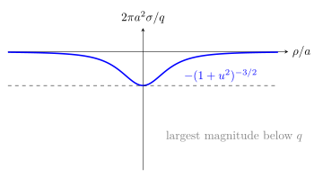
图 7 的横坐标可取有符号径向剖面;真实轴对称密度只依赖 \(\rho\ge0\)。
3.3 Force and energy caveat
真实电荷所受力可直接视为 image charge 的 Coulomb force。但能量必须计
\[U=\frac12qV_{\mathrm{image}}(\mathbf r_q),\]
因为感应电荷随真实电荷从无穷远移入而逐步建立;漏掉 \(1/2\) 会把能量算成两倍。
Knowledge 4 — Electric and magnetic multipole expansions / 电与磁多极展开
Knowledge ID: P04-U11-L01-K04
4.1 Electric expansion
对局域电荷源且 \(r>a\),展开 Coulomb kernel:
\[V(\mathbf r)=\frac{1}{4\pi\epsilon_0} \left[ \frac{Q}{r} +\frac{\mathbf p\cdot\hat{\mathbf r}}{r^2} +\frac{1}{2r^3}Q_{ij}\hat r_i\hat r_j +\cdots \right],\]
其中采用求和约定,且
\[Q=\int\rho\,d\tau',\qquad \mathbf p=\int\rho\,\mathbf r'\,d\tau',\]
\[Q_{ij}=\int\rho(\mathbf r') \left(3x_i'x_j'-r'^2\delta_{ij}\right)d\tau'.\]
最低非零矩控制远场:monopole 势按 \(r^{-1}\),dipole 按 \(r^{-2}\),quadrupole 按 \(r^{-3}\)。若 \(Q\neq0\),\(\mathbf p\) 会随原点平移;若 \(Q=0\),\(\mathbf p\) 与原点无关。
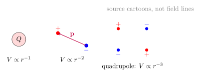
图 8 将各阶与远场幂律对应;复杂源只有在低阶矩因对称性为零时才由更高阶主导。
4.2 Magnetic expansion
这里采用磁静力学矢势(magnetostatic vector potential)\(\mathbf A\),定义为满足 \(\mathbf B=\nabla\times\mathbf A\) 的矢量场;同一 \(\mathbf B\) 可对应多个 \(\mathbf A\),其 gauge freedom 留到 Potentials and Gauge Freedom 系统讨论。
稳恒局域电流没有磁单极项。其领先 far-field moment 为
\[\mathbf m=\frac12\int\mathbf r'\times\mathbf J(\mathbf r')\,d\tau',\]
对应
\[\mathbf A(\mathbf r)\simeq \frac{\mu_0}{4\pi}\frac{\mathbf m\times\hat{\mathbf r}}{r^2},\]
\[\mathbf B(\mathbf r)\simeq \frac{\mu_0}{4\pi r^3} \left[3(\mathbf m\cdot\hat{\mathbf r})\hat{\mathbf r}-\mathbf m\right].\]
平面细线回路给 \(\mathbf m=IA\hat{\mathbf n}\)。
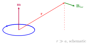
图 9 表示电流环到磁偶极描述的尺度压缩;近环场不能由该图外推。
4.3 Method selection
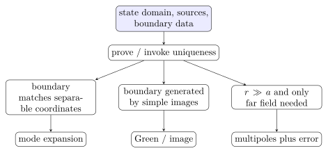
图 10 表示方法不是互斥的:Green function 可用 modes 展开,image 是特殊 Green construction,multipoles 可再压缩其远场。
Worked Examples / 完整例题
Worked Example 1 — One mode in a rectangle / 矩形中的单一模式
已知: \(0<x<a=0.200\ \mathrm m\)、\(0<y<b=0.100\ \mathrm m\);除 \(y=0\) 外三边接地,底边 \(V(x,0)=100\sin(\pi x/a)\ \mathrm V\)。求 \((x,y)=(0.100,0.0400)\ \mathrm m\) 的 \(V\) 与 \(\mathbf E\)。
系统、坐标与模型: 矩形内部无电荷,二维 Laplace equation;边界恰是第一 sine mode。
\[V=100\sin\frac{\pi x}{a} \frac{\sinh[\pi(b-y)/a]}{\sinh(\pi b/a)}.\]
在 \(x=a/2\),\(\sin(\pi x/a)=1\)、\(\cos(\pi x/a)=0\):
\[V=100\frac{\sinh(0.9425)}{\sinh(1.571)} =47.3\ \mathrm V, \qquad E_x=-\frac{\partial V}{\partial x}=0.\]
\[E_y=-\frac{\partial V}{\partial y} =\frac{100\pi}{a} \frac{\cosh[\pi(b-y)/a]}{\sinh(\pi b/a)} =1.01\times10^3\ \mathrm{V\,m^{-1}}.\]
检查: \(0<V<100\ \mathrm V\);向上接近接地边界时势下降,所以 \(E_y>0\)。边界和单位一致。
Worked Example 2 — Charge above a grounded plane / 接地平面上方点电荷
已知: \(q=5.00\ \mathrm{nC}\) 位于 \(z=a=3.00\ \mathrm{cm}\)。求静电吸引力与相对无穷远的系统能量。
系统与模型: 真实系统是点电荷加接地导体;在 \(z>0\) 用 \(-q\) image。\(+z\) 远离平面。
image 与真实电荷相距 \(2a\):
\[\mathbf F=-\frac{1}{4\pi\epsilon_0}\frac{q^2}{(2a)^2}\hat{\mathbf z} =-6.24\times10^{-5}\hat{\mathbf z}\ \mathrm N.\]
能量不是真实—image 两电荷的完整 Coulomb 能,而是
\[U=\frac12qV_{\mathrm{image}}(\mathbf r_q) =-\frac{q^2}{16\pi\epsilon_0a} =-1.87\times10^{-6}\ \mathrm J.\]
检查: \(-\partial U/\partial a=-q^2/(16\pi\epsilon_0a^2)\),与力一致;漏掉 \(1/2\) 会破坏此检查。
Worked Example 3 — Electric dipole far field / 电偶极远场
已知: \(+3.00\ \mathrm{nC}\) 位于 \(z=+2.00\ \mathrm{cm}\),\(-3.00\ \mathrm{nC}\) 位于 \(z=-2.00\ \mathrm{cm}\)。求 \(+z\) 轴 \(r=0.500\ \mathrm m\) 的 dipole potential。
源、原点与模型: 原点在两电荷中点,净电荷 \(Q=0\);最大源坐标 \(a=0.0200\ \mathrm m\),\(a/r=0.0400\)。
\[\mathbf p=q(0.0400\ \mathrm m)\hat{\mathbf z} =1.20\times10^{-10}\hat{\mathbf z}\ \mathrm{C\,m}.\]
\[V_{\mathrm{dip}}=\frac{1}{4\pi\epsilon_0}\frac{p}{r^2} =4.31\ \mathrm V.\]
检查: \(r/a=25\),下一非零相对修正为 \(O[(a/r)^2]\);\(+z\) 轴靠近正电端,势应为正。
Worked Example 4 — Magnetic loop far field / 磁环远场
已知: 圆环 \(I=2.00\ \mathrm A\)、\(R=3.00\ \mathrm{cm}\),求赤道面 \(r=0.400\ \mathrm m\) 处的偶极场。
系统与模型: \(\mathbf m\) 沿 \(+z\);\(R/r=0.0750\ll1\),观察点在 \(\mathbf m\cdot\hat{\mathbf r}=0\) 的赤道面。
\[m=I\pi R^2=5.65\times10^{-3}\ \mathrm{A\,m^2}.\]
\[\mathbf B_{\mathrm{eq}} =-\frac{\mu_0m}{4\pi r^3}\hat{\mathbf z} =-8.84\times10^{-9}\hat{\mathbf z}\ \mathrm T.\]
检查: 赤道场与 \(\mathbf m\) 反向,单位为 T,且 \(r\) 增大时按 \(r^{-3}\) 衰减。
Lesson synthesis / 本课综合
边值问题的首要对象是“域 + 源 + 边界数据”,而不是孤立微分方程。Uniqueness theorem 让正确构造升级为唯一物理解;separation 将边界展开为本征模式;Green function 是边界适配点响应,image method 是其特殊构造;multipole expansion 则在 \(a/r\ll1\) 时只保留少量远场矩。四种方法通过边界、尺度和所需输出互相衔接。
Formula-and-decision table / 公式与决策表
| Goal | Method / formula | Conditions and checks |
|---|---|---|
| Establish unique electrostatic solution | difference solution + Green first identity | Dirichlet; Neumann up to constant |
| Solve regular coordinate boundary | \(V=\sum X_nY_nZ_n\) | separable geometry and complete eigenbasis |
| Build response for arbitrary source | Green representation | state normalization and boundary rule for \(G\) |
| Replace simple grounded conductor | image charges | images outside physical domain; invoke uniqueness |
| Force in image problem | Coulomb force from images | force on real charges only |
| Energy in image problem | \(U=\tfrac12\sum q_iV_{\mathrm{image}}(\mathbf r_i)\) | induced charges; avoid double counting |
| Far electric field | monopole, dipole, quadrupole series | \(a/r\ll1\); track origin dependence |
| Far magnetic field | \(\mathbf m=\tfrac12\int\mathbf r'\times\mathbf J\,d\tau'\) | localized steady current; no magnetic monopole |
Model boundaries / 模型边界
- Uniqueness assumes specified domain, regularity and consistent boundary data; Neumann data require compatibility.
- Separation of variables depends on separable coordinates and a complete basis; irregular geometries often need numerical methods.
- Point sources and perfect sharp conductors create mathematical singularities; finite source size and rounded edges regularize reality.
- Image charges solve only the stated boundary and physical domain; they cannot be used as real internal charge distributions.
- Multipoles converge outside a sphere containing all sources; near field or extended nonlocal sources may not admit useful truncation.
- Static electric and magnetic multipoles are not yet radiation multipoles; time dependence adds retardation and gauge structure.
Misconception clinic / 误区诊所
- “满足 Laplace equation 就是答案。” 没有边界数据,存在无穷多个解。
- Neumann problem 与 Dirichlet 一样绝对唯一。 Neumann 解可加常数,且数据须满足 compatibility。
- 分离变量只能给单个乘积。 一般边界需要本征函数叠加;单乘积只是 basis mode。
- Image charge 在导体内部真实存在。 它是被排除域中的数学构造。
- image 能量直接用 \(qV_{\mathrm{image}}\)。 感应边界问题必须乘 \(1/2\)。
- dipole moment 总与原点无关。 只有总电荷为零时才与原点无关。
- 远场只看源到观察点距离大。 必须与源尺寸比较,即 \(a/r\ll1\)。
- 磁 multipole 也从 monopole 开始。 经典 Maxwell theory 中 \(\nabla\cdot\mathbf B=0\),局域稳恒电流的领先项是 dipole。
Practice and retrieval / 练习与提取
- 唯一性(K01): 为什么 Dirichlet 差函数证明中的 \(\int\lvert\nabla U\rvert^2d\tau=0\) 能推出 \(U=0\)?
- Neumann(K01): 写出 Poisson problem 的 Neumann compatibility condition,并说明剩余自由度。
- 矩形模式(K02): 在三边接地矩形中,底边为 \(V_0\sin(2\pi x/a)\),写出解。
- 坐标选择(K02): 球面边界且轴对称时,为何 Legendre polynomials 比 Cartesian sine modes 自然?
- Green convention(K03): 本课 \(G\) 的微分方程是什么?它的单位是什么?
- Image surface charge(K03): 接地点电荷问题中,\(\sigma(\rho)\) 的符号为何处处为负?总感应电荷是多少?
- Image energy(K03): 解释 energy expression 中因子 \(1/2\) 的物理来源。
- Electric multipole(K04): 净电荷为零且 \(\mathbf p=0\) 的局域源,领先势通常按什么幂衰减?
- Origin shift(K04): 总电荷 \(Q\neq0\) 时将原点平移 \(\mathbf a\),\(\mathbf p\) 如何变化?
- Magnetic dipole(K04): 电流环半径减半、电流不变,固定远场点的 dipole field 变为原来的多少?
Answer
被积函数处处非负;在连续或分段光滑条件下,积分为零迫使 \(\nabla U=0\)。故 \(U\) 为常数,Dirichlet 零边界再迫使常数为零。
Answer
必须满足 \(\int_{\partial\Omega}(\partial V/\partial n)\,da=-\epsilon_0^{-1}\int_\Omega\rho\,d\tau\);满足后,\(V\) 仍可整体加任意常数。
Answer
分离变量给出 \(V=V_0\sin(2\pi x/a)\sinh[2\pi(b-y)/a]/\sinh(2\pi b/a)\);它在 \(y=b\) 恢复给定正弦边界,在 \(y=0\) 为零。
Answer
球面是 spherical coordinates 的坐标面,角向 Laplace operator 的轴对称本征函数正是 \(P_\ell(\cos\theta)\),因此边界匹配与正交展开都直接。
Answer
本课约定 \(\nabla'^2G=-4\pi\delta(\mathbf r-\mathbf r')\)。因 Laplacian 的量纲为 \(\mathrm{m^{-2}}\)、delta 为 \(\mathrm{m^{-3}}\),故 \(G\) 的单位为 \(\mathrm{m^{-1}}\)。
Answer
\(\sigma(\rho)=-qa/[2\pi(\rho^2+a^2)^{3/2}]<0\),所以符号处处为负;对整个平面积分得到总感应电荷 \(-q\)。
Answer
导体的感应电荷随真实电荷从无穷远移入而逐步建立,沿准静态装配路径的平均 interaction potential 是终值的一半;等价地,因子 \(1/2\) 避免把感应相互作用重复计数。
Answer
通常由 quadrupole 主导,\(V\propto r^{-3}\);若 quadrupole 也因对称性为零,则由更高阶主导并衰减更快。
Answer
若新坐标为 \(\mathbf r''=\mathbf r'-\mathbf a\),则 \(\mathbf p''=\int\mathbf r''\rho\,d\tau'=\mathbf p-Q\mathbf a\),单位仍为 \(\mathrm{C\,m}\)。
Answer
\(m=I\pi R^2\);半径减半使 \(m\) 变为原来的 \(1/4\),所以在固定远场点 \(\mathbf B\) 也变为原来的 \(1/4\)。
Exit ticket / 离堂检核
- 对“点电荷在接地平面上方”的问题,按逻辑顺序写出 image construction、边界核验、唯一性论证、force 与 energy 的区别。
- 一个中性局域源的 dipole moment 也为零。说明观察距离加倍时其领先 potential 与 electric field 各缩小多少倍。
References and source notes / 参考资料与来源说明
Source-to-content map
| Source | Used for | Knowledge ID / section | Model boundary or convention |
|---|---|---|---|
| MIT OCW 8.07, Lecture Notes 5: Method of Images and Separation of Variables | image method, separable electrostatic geometries | K01–K03 | conductor boundaries and uniqueness |
| MIT OCW 8.07, Lecture Notes 9: Traceless Symmetric Tensor Approach to Legendre Polynomials and Spherical Harmonics (§7 The Multipole Expansion) | electric multipole expansion and moments | K04 | far-field series and conventions |
| MIT OCW 8.07, Lecture Notes 10: Magnetic Multipoles | magnetic dipole moment and vector potential | K04 | localized steady currents |
| University of Virginia, Electrostatics II | Green identities, Green functions, Dirichlet/Neumann uniqueness | K01, K03 | Green-function normalization checked |
| MIT OCW 6.641, Lecture 5: Method of Images | grounded-conductor image constructions | K03 | images restricted to excluded domain |
| University of Virginia, Magnetostatics II | \(\mathbf m=\tfrac12\int\mathbf r'\times\mathbf J\,d\tau'\) and far \(\mathbf A\) | K04 | SI magnetic multipole convention |
资料与链接实际浏览、阅读和核对日期:2026-08-28。Green function 的 \(4\pi\) normalization 已在正文显式声明;全部图为基于方程的原创示意。
复习与拓展
- Potentials and Gauge Freedom:Green functions 与 potentials 的 gauge structure。
- Radiation theory:把 static multipoles 推广为 time-dependent radiation multipoles。
- Numerical electromagnetism:有限差分、有限元与 boundary element method。
- Mathematical physics:self-adjoint operators、spectral expansions 与 reciprocity。