势与规范自由 · Potentials and Gauge Freedom

Learning objectives / 学习目标

完成本课后，你应能：

由 $\nabla\cdot\mathbf B=0$ 与 Faraday law 构造 $\Phi,\mathbf A$ ，并从势恢复 $\mathbf E,\mathbf B$ ；
证明 $\mathbf A'=\mathbf A+\nabla\chi$ 、 $\Phi'=\Phi-\partial\chi/\partial t$ 不改变场；
比较 Coulomb gauge 与 Lorenz gauge 的约束、方程、优势及残余规范自由；
从 Lorenz-gauge wave equations 写出 retarded potentials，解释延迟时刻与因果边界条件；
区分 gauge-dependent 中间量与 gauge-invariant fields、Lorentz force、flux、能量流及闭合相位。

Prerequisites / 先修知识

Maxwell's Completion of Electromagnetism：完整 Maxwell 方程与连续性方程。
Boundary-Value and Multipole Methods：Poisson equation、Green function 与边界条件。
vector identities： $\nabla\cdot(\nabla\times\mathbf A)=0$ 、 $\nabla\times(\nabla\chi)=0$ 。
wave operator、延迟 Green function 与局域电荷守恒。

Scope and conventions / 范围与约定

采用 SI 与 $\mathbf E=-\nabla\Phi-\partial\mathbf A/\partial t$ ， $\mathbf B=\nabla\times\mathbf A$ 。
wave operator 写为 $\Box=\nabla^2-c^{-2}\partial_t^2$ ，故 Lorenz gauge 中 $\Box\Phi=-\rho/\epsilon_0$ 、 $\Box\mathbf A=-\mu_0\mathbf J$ 。
Lorenz gauge 以 Ludvig Lorenz 命名，不写成 Lorentz gauge；Lorentz 指变换/力等其他概念。
假设源 $\rho,\mathbf J$ 满足 $\partial_t\rho+\nabla\cdot\mathbf J=0$ ，且空间无磁单极子。
retarded solution 还需“无来自过去无穷远的入射齐次波”等边界条件；微分方程本身也允许 advanced 或任意齐次解。
quantum phase 只作为 gauge-invariant observable 的接口，不展开量子动力学。
TikZ 均为 schematic / not to scale。

Notation and modeling contract / 符号与建模契约

Symbol	Meaning	SI unit
$\Phi$	scalar potential	V
$\mathbf A$	vector potential	$\mathrm{V\,s\,m^{-1}}=\mathrm{T\,m}$
$\chi$	gauge function	$\mathrm{V\,s}$
$\Box$	$\nabla^2-c^{-2}\partial_t^2$	operator
$\mathbf R=\mathbf r-\mathbf r'$	source-to-observer displacement	m
$$t_r=t-R/c$$	retarded time	s
$A^\mu,J^\mu$	four-potential and four-current	convention-dependent components

Knowledge 1 — Scalar and vector potentials / 标势与矢势

Knowledge ID: P04-U11-L02-K01

由于 $\nabla\cdot\mathbf B=0$ ，在单连通局部区域可写

$\mathbf B=\nabla\times\mathbf A.$

代入 Faraday law：

$\nabla\times\left(\mathbf E+\frac{\partial\mathbf A}{\partial t}\right)=0.$

故括号内可写成某标量的负梯度：

$\boxed{\mathbf E=-\nabla\Phi-\frac{\partial\mathbf A}{\partial t}}, \qquad \boxed{\mathbf B=\nabla\times\mathbf A}.$

静电学的 $\mathbf E=-\nabla\Phi$ 只是 $\partial_t\mathbf A=0$ 的特殊情形；时变电磁场不能只靠标势。

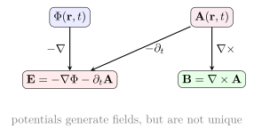
Potentials and Gauge Freedom — Knowledge 1 — Scalar and vector potentials / 标势与矢势（图 1） — 图 1Knowledge 1 — Scalar and vector potentials / 标势与矢势

图 1 展示势到场的微分映射。由 4 个势分量得到 6 个场分量并不矛盾，因为场满足两条 homogeneous Maxwell constraints，而势还含一函数的冗余。

势的单位检查： $\partial_t\mathbf A$ 必须与 $\mathbf E$ 同单位，故 $[\mathbf A]=\mathrm{V\,s\,m^{-1}}$ ； $\nabla\times\mathbf A$ 的单位为 T。

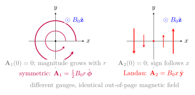
Potentials and Gauge Freedom — Knowledge 1 — Scalar and vector potentials / 标势与矢势（图 2） — 图 2Knowledge 1 — Scalar and vector potentials / 标势与矢势

图 2 用并列 $$x$$ – $$y$$ 面板比较两套 gauge fields：symmetric gauge 的 $\mathbf A_1$ 沿圆周切向且大小随半径增长；Landau gauge 的 $\mathbf A_2$ 沿 $$y$$ 方向、正负由 $$x$$ 决定，并在 $$x=0$$ 消失。两者都在原点给 $\mathbf A=0$ ，而 curl 均为同一出纸面的 $B_0\hat{\mathbf z}$ 。

Knowledge 2 — Gauge transformations / 规范变换

Knowledge ID: P04-U11-L02-K02

对任意足够光滑的标量函数 $\chi(\mathbf r,t)$ ，定义

$\mathbf A'=\mathbf A+\nabla\chi, \qquad \Phi'=\Phi-\frac{\partial\chi}{\partial t}.$

则

$\mathbf B'=\nabla\times\mathbf A' =\mathbf B+\nabla\times\nabla\chi=\mathbf B,$

$\mathbf E'=-\nabla\Phi'-\partial_t\mathbf A' =\mathbf E+\nabla\partial_t\chi-\partial_t\nabla\chi =\mathbf E.$

这叫 gauge transformation。它不是把一个物理场变成另一个物理场，而是在同一物理等价类中换代表元。

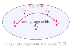
Potentials and Gauge Freedom — Knowledge 2 — Gauge transformations / 规范变换（图 3） — 图 3Knowledge 2 — Gauge transformations / 规范变换

图 3 把规范选择画成“坐标冗余的轨道”；选择 gauge 类似从轨道中挑一个计算方便的点。

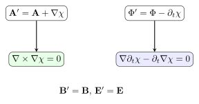
Potentials and Gauge Freedom — Knowledge 2 — Gauge transformations / 规范变换（图 4） — 图 4Knowledge 2 — Gauge transformations / 规范变换

图 4 分别指出 $\mathbf B$ 不变来自 curl-grad identity，而 $\mathbf E$ 不变依赖时空偏导可交换。

规范条件通常不能完全消除自由。若已经在 Lorenz gauge，仍可做满足 $\Box\chi=0$ 的 residual gauge transformation；还需边界/初始条件才可能唯一选定代表元。

Knowledge 3 — Coulomb and Lorenz gauges / 库仑规范与洛伦兹规范

Knowledge ID: P04-U11-L02-K03

把 Maxwell 方程写成势后仍是耦合方程。Gauge freedom 允许选择约束来简化它们。

Coulomb gauge

$\nabla\cdot\mathbf A=0.$

Gauss law 立即给

$\nabla^2\Phi=-\frac{\rho}{\epsilon_0}.$

它在每一时刻看似 Poisson equation，适合准静态、边值与 transverse/longitudinal 分解。这里 $\Phi$ 的“瞬时”形式不意味着可超光速通信： $-\nabla\Phi$ 中看似瞬时的部分与 $-\partial_t\mathbf A$ 的相应部分在 $\mathbf E$ 中抵消，最终场保持因果。

Lorenz gauge

$\nabla\cdot\mathbf A+\frac{1}{c^2}\frac{\partial\Phi}{\partial t}=0.$

势方程解耦为

$\Box\Phi=-\frac{\rho}{\epsilon_0}, \qquad \Box\mathbf A=-\mu_0\mathbf J.$

它显式保持相对论协变结构，并自然导向 retarded potentials。连续性方程保证这两个有源波动方程与 gauge condition 相容。

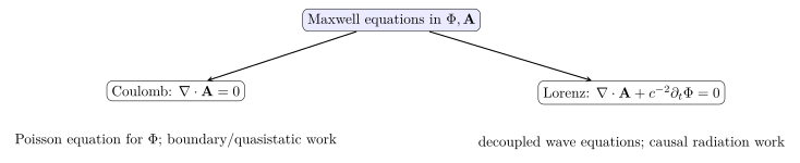
Potentials and Gauge Freedom — Lorenz gauge（图 5） — 图 5Lorenz gauge

图 5 比较两种 gauge 的计算功能，不把其中任何一种说成“更真实”。

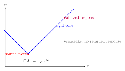
Potentials and Gauge Freedom — Lorenz gauge（图 6） — 图 6Lorenz gauge

图 6 显示 Lorenz-gauge wave equation 的特征锥；因果性还需选择 retarded 而非 advanced Green function。

Knowledge 4 — Retarded potentials / 推迟势

Knowledge ID: P04-U11-L02-K04

定义

$\mathbf R=\mathbf r-\mathbf r', \qquad R=\lvert\mathbf R\rvert, \qquad t_r=t-\frac{R}{c}.$

在自由空间 retarded boundary condition 下，Lorenz-gauge 解为

$\boxed{\Phi(\mathbf r,t)=\frac{1}{4\pi\epsilon_0} \int\frac{\rho(\mathbf r',t_r)}{R}\,d^3r'},$

$\boxed{\mathbf A(\mathbf r,t)=\frac{\mu_0}{4\pi} \int\frac{\mathbf J(\mathbf r',t_r)}{R}\,d^3r'}.$

每个源元的延迟不同，因为 $$R$$ 随 $\mathbf r'$ 变化；不能在扩展源中用一个共同 $$t-r/c$$ ，除非远场近似已被证明。

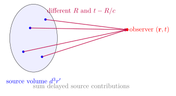
Potentials and Gauge Freedom — Knowledge 4 — Retarded potentials / 推迟势（图 7） — 图 7Knowledge 4 — Retarded potentials / 推迟势

图 7 表示 retarded integral 是对“不同过去时刻”的源求和，不是同一时刻的 Coulomb 叠加。

波动方程还允许 advanced solution $$t_a=t+R/c$$ ，也允许加任意无源齐次波。通常选择 retarded solution 是物理边界条件：场由过去的源产生，且没有从未来或过去无穷远专门汇聚来的波。

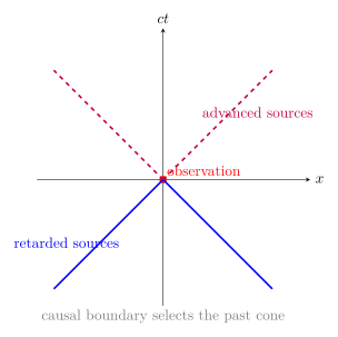
Potentials and Gauge Freedom — Knowledge 4 — Retarded potentials / 推迟势（图 8） — 图 8Knowledge 4 — Retarded potentials / 推迟势

图 8 区分数学允许性与通常的因果物理选择；“retarded”不由 gauge condition 单独保证。

Knowledge 5 — Gauge-invariant fields and observables / 规范不变的场与可观测量

Knowledge ID: P04-U11-L02-K05

经典局域可观测量由 $\mathbf E,\mathbf B$ 构成，例如 Lorentz force density、能量密度、Poynting vector 与应力。它们在 gauge transformation 下不变：

$\mathbf f=\rho\mathbf E+\mathbf J\times\mathbf B, \qquad u=\frac{\epsilon_0E^2}{2}+\frac{B^2}{2\mu_0}, \qquad \mathbf S=\frac{1}{\mu_0}\mathbf E\times\mathbf B.$

势本身依赖 gauge，但某些闭合/拓扑组合可规范不变。静态 gauge function 单值时，

$\oint_C\mathbf A'\cdot d\boldsymbol\ell =\oint_C\mathbf A\cdot d\boldsymbol\ell +\oint_C\nabla\chi\cdot d\boldsymbol\ell =\oint_C\mathbf A\cdot d\boldsymbol\ell =\Phi_B.$

在量子力学中，相位差含 $q\oint\mathbf A\cdot d\boldsymbol\ell/\hbar$ ；Aharonov–Bohm geometry 展示即使粒子路径上的 $\mathbf B=0$ ，被两路径围住的磁通仍可改变干涉相位。可观测的是闭合相位/磁通，不是某一 gauge 下单点 $\mathbf A$ 的数值。

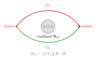
Potentials and Gauge Freedom — Knowledge 5 — Gauge-invariant fields and observables / 规范不变的场与可观测量（图 9） — 图 9Knowledge 5 — Gauge-invariant fields and observables / 规范不变的场与可观测量

图 9 是拓扑接口示意；本课不推导完整量子传播子，只强调 observable 必须对 gauge choice 不变。

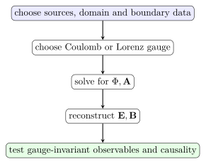
Potentials and Gauge Freedom — Knowledge 5 — Gauge-invariant fields and observables / 规范不变的场与可观测量（图 10） — 图 10Knowledge 5 — Gauge-invariant fields and observables / 规范不变的场与可观测量

图 10 是势方法的审计流程：不能把“求出某个 $\mathbf A$ ”当作终点，必须还原场并检查可观测量。

Worked Examples / 完整例题

Worked Example 1 — Trading a time-dependent vector potential for a scalar potential / 交换势的角色

已知条件： 均匀电场 $\mathbf E=E_0\hat{\mathbf x}$ 、 $\mathbf B=0$ 。一种势为 $\Phi=0$ 、 $\mathbf A=-E_0t\hat{\mathbf x}$ 。
研究对象与边界： 全空间局部区域；求 gauge function 使 $\mathbf A'=0$ 。
参考系与正方向： 给定实验室系， $$+x$$ 沿电场。
模型及理由： 场均匀、偏导可交换、区域单连通。

选

$\chi=E_0tx.$

则

$\nabla\chi=E_0t\hat{\mathbf x}, \qquad \mathbf A'=\mathbf A+\nabla\chi=0,$

$\Phi'=\Phi-\partial_t\chi=-E_0x.$

恢复场：

$\mathbf E'=-\nabla\Phi'-\partial_t\mathbf A'=E_0\hat{\mathbf x}, \qquad \mathbf B'=0.$

结论： 同一均匀电场可由纯时变矢势或纯空间标势表示。
检查： $[\chi]=[E_0tx]=\mathrm{V\,s}$ ； $\mathbf E',\mathbf B'$ 与原场一致。若只改 $\mathbf A$ 不同时改 $\Phi$ ，会错误改变电场。

Worked Example 2 — Two gauges for a uniform magnetic field / 均匀磁场的两种规范

已知条件： $\mathbf B=B_0\hat{\mathbf z}$ 。给出 symmetric gauge $\mathbf A_1=(-B_0y/2,B_0x/2,0)$ 与 Landau gauge $\mathbf A_2=(0,B_0x,0)$ 。
研究对象与边界： 全空间局部区域；寻找 $\chi$ 使 $\mathbf A_2=\mathbf A_1+\nabla\chi$ 。
参考系与正方向： Cartesian $$x,y,z$$ 。
模型及理由： 静态、单连通区域。

差为

$\mathbf A_2-\mathbf A_1=\left(\frac{B_0y}{2},\frac{B_0x}{2},0\right).$

取

$\chi=\frac{B_0xy}{2},$

则 $\nabla\chi$ 正是上述差。两者的 curl 均为

$\nabla\times\mathbf A_1=\nabla\times\mathbf A_2=B_0\hat{\mathbf z}.$

结论： 两套不同的 $\mathbf A$ 属于同一 gauge orbit。
检查： $$B_0xy$$ 单位 $\mathrm{T\,m^2}=\mathrm{V\,s}$ ； $\partial_xA_y-\partial_yA_x=B_0$ 。这也解释为何图形外观不同不能当作磁场不同。

Worked Example 3 — Retarded contribution from one source cell / 单个源元的推迟贡献

已知条件： 某守恒扩展源中的一个小体元在 $\mathbf r'=0$ 的电荷贡献为 $\Delta q(t)=q_0\cos(2\pi ft)$ ， $q_0=1.00\ \mathrm{nC}$ 、 $f=10.0\ \mathrm{MHz}$ ；观察点距离 $R=6.00\ \mathrm m$ ，求 $$t=0$$ 时该体元对 $\Phi$ 的 retarded integrand contribution。取 $c=3.00\times10^8\ \mathrm{m\,s^{-1}}$ 。
研究对象与边界： 只计算 Green-function 积分中此体元项；源其余部分与电流保证整体连续性。
参考系与正方向： 源与观察者静止的实验室系。
模型及理由： 自由空间 Lorenz gauge、点状体元近似。

$R/c=\frac{6.00}{3.00\times10^8}=20.0\ \mathrm{ns}.$

$\Delta q(t_r)=q_0\cos[-2\pi(10.0\times10^6)(20.0\times10^{-9})] =q_0\cos(-0.4\pi)=0.309q_0.$

$\Delta\Phi=\frac{1}{4\pi\epsilon_0}\frac{0.309\times10^{-9}}{6.00} =0.463\ \mathrm V.$

结论： 该体元在 $$t=0$$ 的 retarded scalar-potential contribution 为 $0.463\ \mathrm V$ 。
检查： 使用的是 $t_r=-20.0\ \mathrm{ns}$ 而非 $$t=0$$ ；相位延迟为周期的 $$0.200$$ 。单个体元电荷随时间变化不能独立存在，必须与周围 $\mathbf J$ 和其他 $\rho$ 一起满足 continuity equation。

Worked Example 4 — Plane-wave potential and gauge-invariant fields / 平面波势与不变量场

已知条件： $\Phi=0$ ， $\mathbf A=A_0\cos(kz-\omega t)\hat{\mathbf x}$ ， $A_0=2.00\times10^{-9}\ \mathrm{V\,s\,m^{-1}}$ ， $f=100\ \mathrm{MHz}$ ， $k=\omega/c$ 。
研究对象与边界： 真空平面波；求场峰值并验证 Lorenz gauge。
参考系与正方向： 波沿 $$+z$$ ， $\mathbf A$ 沿 $$+x$$ 。
模型及理由： 无源真空、单色平面波。

因 $$A_z=0$$ 且 $$A_x$$ 不依赖 $$x$$ ， $\nabla\cdot\mathbf A=0$ ；又 $\partial_t\Phi=0$ ，故满足 Lorenz gauge。

$\mathbf E=-\partial_t\mathbf A =-\omega A_0\sin(kz-\omega t)\hat{\mathbf x},$

$\mathbf B=\nabla\times\mathbf A =-kA_0\sin(kz-\omega t)\hat{\mathbf y}.$

$E_0=\omega A_0=2\pi(100\times10^6)(2.00\times10^{-9})=1.26\ \mathrm{V\,m^{-1}},$

$B_0=kA_0=\frac{E_0}{c}=4.19\times10^{-9}\ \mathrm T.$

结论： $E_0=1.26\ \mathrm{V\,m^{-1}}$ ， $B_0=4.19\ \mathrm{nT}$ ，且 $$E_0/B_0=c$$ 。
检查： $\mathbf E\times\mathbf B$ 沿 $$+z$$ （两者同时带相同负号），能流方向与相位 $kz-\omega t$ 一致。任何 gauge transform 会改变势但不改变这些场峰值。

Lesson synthesis / 课程综合

势方法的逻辑链为：

homogeneous Maxwell equations 保证可引入 $\Phi,\mathbf A$ ；
引入势产生一函数的 gauge redundancy；
选择 Coulomb 或 Lorenz gauge 简化有源方程，而非改变物理；
Lorenz gauge 加 retarded boundary condition 给因果势积分；
最终预测必须用 gauge-invariant fields、forces、energy flux、fluxes 或闭合相位检验。

Formula-and-decision table / 公式与决策表

Task	Formula / choice	Conditions / caution
从势求场	$\mathbf B=\nabla\times\mathbf A$ ， $\mathbf E=-\nabla\Phi-\partial_t\mathbf A$	两项必须同时保留
换规范	$\mathbf A'=\mathbf A+\nabla\chi$ ， $\Phi'=\Phi-\partial_t\chi$	$\chi$ 足够光滑；边界也需转换
准静态/边值	Coulomb gauge $\nabla\cdot\mathbf A=0$	$\Phi$ 看似瞬时不代表场超光速
辐射/相对论	Lorenz gauge $\nabla\cdot\mathbf A+c^{-2}\partial_t\Phi=0$	仍有 $\Box\chi=0$ residual freedom
自由空间因果解	retarded potentials	还需过去边界条件与 conserved sources
检查物理	重建 $\mathbf E,\mathbf B$ 与 observables	单个势分量通常非 observable

Model boundaries / 模型边界

$\mathbf B=\nabla\times\mathbf A$ 的全局表示可能受区域拓扑影响；局部总可用，非单连通区域需拼接或考虑 holonomy。
Gauge choice 不是边界条件；Lorenz gauge 不自动排除 advanced wave。
Retarded integrals假定自由空间 Green function；导体、介质或腔体要用符合其边界的 Green function。
Coulomb-gauge $\Phi$ 的瞬时 Poisson 形式不能单独解释信号；只有完整 $\mathbf E$ 可观测。
Aharonov–Bohm 讨论依赖量子相位与单值性条件，本课只作后续接口。

Misconception clinic / 误区诊所

“规范变换改变了场。” 若 $\Phi$ 与 $\mathbf A$ 成对变换， $\mathbf E,\mathbf B$ 精确不变。
“Lorenz gauge 是 Lorentz 发明/命名。” 名称来自 Ludvig Lorenz；它恰好具有 Lorentz-covariant 形式。
“Coulomb gauge 违反相对论因果性。” 单独的 $\Phi$ 看似瞬时；与 $-\partial_t\mathbf A$ 合成的 $\mathbf E$ 保持因果。
“波动方程唯一给 retarded solution。” 还可有 advanced 与齐次解；物理边界条件选择 retarded。
“势完全不可观测，所以没有意义。” 单点势依赖 gauge，但闭合相位、flux linkage 与量子干涉等 gauge-invariant 组合有物理意义。

Practice and retrieval / 练习与检索

[P04-U11-L02-K01] 若 $\mathbf A=(-By/2,Bx/2,0)$ ，求 $\mathbf B$ 。

Answer

$B_z=\partial_xA_y-\partial_yA_x=B/2-(-B/2)=B$ ，其余分量为零，所以 $\mathbf B=B\hat{\mathbf z}$ 。

[P04-U11-L02-K01] 为什么时变场中不能普遍写 $\mathbf E=-\nabla\Phi$ ？

Answer

因 Faraday law 允许 $\nabla\times\mathbf E\ne0$ ；必须加入 $-\partial_t\mathbf A$ 才能产生非零 curl。

[P04-U11-L02-K02] 证明 time-independent $\chi$ 不改变 $\Phi$ ，但仍可改变 $\mathbf A$ 。

Answer

$\partial_t\chi=0$ ，故 $\Phi'=\Phi$ ；若 $\nabla\chi\ne0$ ，则 $\mathbf A'=\mathbf A+\nabla\chi$ 。其 curl 仍不变。

[P04-U11-L02-K02] Lorenz gauge 下怎样的 residual $\chi$ 保持 gauge condition？

Answer

代入变换后额外项为 $\Box\chi$ ，所以要求 $\Box\chi=0$ ，并同时满足相关边界/初值条件。

[P04-U11-L02-K03] 写出 Coulomb gauge 与 Lorenz gauge 的条件，并各说一个适合场景。

Answer

Coulomb： $\nabla\cdot\mathbf A=0$ ，适合静电/准静态边值；Lorenz： $\nabla\cdot\mathbf A+c^{-2}\partial_t\Phi=0$ ，适合波动、辐射与协变处理。

[P04-U11-L02-K03] Lorenz gauge 中 $\rho=0,\mathbf J=0$ 时，势满足什么方程？

Answer

$\Box\Phi=0$ 、 $\Box\mathbf A=0$ ；它们可包含自由电磁波，但还须满足 gauge condition 与边界数据。

[P04-U11-L02-K04] 观察点距源元 $300\ \mathrm m$ ，自由空间延迟是多少？

Answer

$R/c=300/(3.00\times10^8)=1.00\ \mu\mathrm s$ ；势在时刻 $$t$$ 使用源元在 $t-1.00\ \mu\mathrm s$ 的值。

[P04-U11-L02-K04] 扩展源为什么不能统一使用 $$t-r/c$$ ？

Answer

每个源点到观察点距离 $R=\lvert\mathbf r-\mathbf r'\rvert$ 不同，故各自 retarded time 不同；只有在受控远场展开下才能近似共同相位。

[P04-U11-L02-K05] 列出三个 gauge-invariant 经典量。

Answer

例如 $\mathbf E$ 、 $\mathbf B$ 、Lorentz force、 $$u$$ 、 $\mathbf S$ 、磁通；任列三项并由场构造即可。

[P04-U11-L02-K05] 为什么 $\oint_C\mathbf A\cdot d\boldsymbol\ell$ 对单值光滑 $\chi$ 的 gauge transform 不变？

Answer

对单值、光滑的 $\chi$ ，规范变换增加的是 exact differential 的闭路积分： $\oint_C\nabla\chi\cdot d\boldsymbol\ell=0,$ 因为 exact differential 绕闭路的首末点相同；等价地， $\nabla\times\nabla\chi=0$ 。另一个独立等式才由 Stokes theorem 给出： $\oint_C\mathbf A\cdot d\boldsymbol\ell =\int_S(\nabla\times\mathbf A)\cdot d\mathbf a =\int_S\mathbf B\cdot d\mathbf a =\Phi_B.$

Exit ticket / 离堂检核

从 $\Phi,\mathbf A$ 的 gauge transform 开始，不跳步证明 $\mathbf E,\mathbf B$ 不变，并说明偏导交换用在何处。
说明 Lorenz gauge、retarded Green function、source continuity 与 causal observable 四者各自承担的不同角色。

References and source notes / 参考资料与来源说明

以下权威直接来源均于 2026-08-28 实际打开核验；不同来源对 $$c$$ 因子与四势分量约定不同，正文统一为 SI 三维形式。

Source-to-content map

Source	Used for	Knowledge ID / Section	Model boundary or convention
MIT 6.013 Lecture 19	potentials, Lorenz-gauge wave equations, retarded solutions	P04-U11-L02-K01, P04-U11-L02-K03, P04-U11-L02-K04	free-space SI and causal boundary
MIT 8.033 notes	gauge transformation proof and covariant structure	P04-U11-L02-K02, P04-U11-L02-K03	derivative and sign convention stated
MIT 8.06 L13.4	gauge equivalence classes and quantum/topological interface	P04-U11-L02-K02, P04-U11-L02-K05	transcript uses a different $$c$$ convention
Feynman Vol. II Ch. 15	vector potential meaning and closed-path phase/flux role	P04-U11-L02-K01, P04-U11-L02-K05	distinguishes gauge-dependent potential from observables
UMD PHYS 411 review	compact SI potential equations and retarded integrals	P04-U11-L02-K03, P04-U11-L02-K04	Lorenz-gauge free-space expressions
Likharev §8.1	Green-function and medium generalization	P04-U11-L02-K04	dispersion-free homogeneous medium before specialization to vacuum

复习与拓展

Radiation from Accelerated Charges 将把 retarded potentials 专门化为移动点电荷的 Liénard–Wiechert potentials。
Energy and Momentum of Electromagnetic Fields 提供 gauge-invariant 能量、动量与 Poynting flux。
后续量子物理会把 $q\mathbf A$ 写入 canonical momentum，并系统处理 Aharonov–Bohm phase。