
Learning objectives / 学习目标
- 在统一笛卡尔坐标下推导并应用球面折射公式。
- 由两个球面折射面得到薄透镜公式、放大率与主光线规则。
- 用曲率半径和相对折射率求 lens-maker equation 与 optical power。
- 逐面追迹多透镜系统,正确处理 intermediate image 作为下一元件的实物或虚物。
- 建立 free propagation 与 thin lens 的 ABCD 矩阵,按光线实际遇到元件的反序书写总乘积。
Prerequisites / 先修知识
- Snell's Law。
- Cartesian Sign Convention and Paraxial Imaging。
- 矩阵乘法不交换:一般 \(M_2M_1\ne M_1M_2\)。
Scope and conventions / 范围与约定
- 光从左向右传播,实验室 \(+x\) 向右;每个折射面顶点或薄透镜主平面作为该步的局部 \(x=0\)。
- 轴上物、像和曲率中心都用 带符号坐标:实物通常 \(x_o<0\),实像通常 \(x_i>0\);曲率中心在表面右侧时 \(R>0\)。
- 横向高度向上为正。对折射面,\(m=n_1x_i/(n_2x_o)\);对两侧同介质的薄透镜,\(m=x_i/x_o\)。
- 薄透镜焦距 \(f>0\) 为会聚、\(f<0\) 为发散;焦距是坐标形式的 signed focal length。
- ABCD 部分采用光线列向量 \((y,\theta)^{\mathsf T}\),仅对同一均匀外介质中的 free space 与 ideal thin lenses 直接使用;角度为小角弧度。
- 元件按 \(M_1,M_2,\ldots,M_N\) 的顺序被光遇到时,总矩阵是 \(M_N\cdots M_2M_1\)。
- 不讨论厚透镜主平面完整求解、高数值孔径、衍射、像差或 Gaussian beam 的复 \(q\) 参数。
Notation and modeling contract / 符号与建模契约
| Symbol | Meaning | SI unit |
|---|---|---|
| \(n_1,n_2\) | refractive indices before and after a surface | 1 |
| \(x_o,x_i\) | local Cartesian object and image coordinates | m |
| \(R,R_1,R_2\) | signed radii; center right of vertex is positive | m |
| \(f\) | signed focal length of a thin lens | m |
| \(\Phi=1/f\) | optical power | \(\mathrm{m^{-1}}=\mathrm D\) |
| \(d\) | axial separation or propagation distance | m |
| \(y,\theta\) | paraxial ray height and slope angle | m, rad |
| \(A,B,C,D\) | entries of a ray-transfer matrix | 1, m, \(\mathrm{m^{-1}}\), 1 |
Knowledge 1 — Refraction at a spherical surface / 球面折射
Knowledge ID: P05-U02-L03-K01
从 Snell 定律到 Gaussian surface equation
球面界面顶点在 \(x=0\),介质 1 在左、介质 2 在右。物点坐标为 \(x_o\),像点为 \(x_i\),曲率中心坐标为 \(R\)。对高度 \(y\) 的近轴光线,所有相关角都小,故 \(\sin\theta\approx\theta\)。
把入射线、法线和折射线相对 \(+x\) 的小斜率代入 \(n_1\theta_1=n_2\theta_2\),整理得到
\[\boxed{\frac{n_2}{x_i}-\frac{n_1}{x_o} =\frac{n_2-n_1}{R}}.\]
这一个式子同时允许实物、虚物、实像、虚像与两种曲率;前提是所有位置都作为坐标代入。
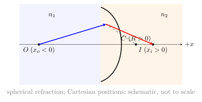
横向放大率来自近轴几何与折射角权重:
\[\boxed{m=\frac{y_i}{y_o}=\frac{n_1x_i}{n_2x_o}}.\]
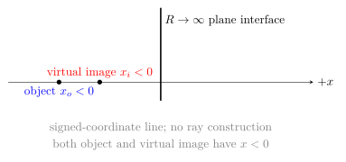
若 \(x_o<0\)、\(x_i>0\),则 \(m<0\),实像倒立。平面界面是 \(R\to\infty\):
\[\frac{n_2}{x_i}=\frac{n_1}{x_o},\]
所以实物 \(x_o<0\) 通常给 \(x_i<0\) 的虚像,这与视深一致。
Knowledge 2 — Thin-lens equation and magnification / 薄透镜公式与放大率
Knowledge ID: P05-U02-L03-K02
两个球面相加
设透镜材料折射率为 \(n_\ell\),外界两侧均为 \(n_m\)。第一表面形成中间像 \(x'\):
\[\frac{n_\ell}{x'}-\frac{n_m}{x_o} =\frac{n_\ell-n_m}{R_1}.\]
在薄透镜极限,两表面顶点视为同一平面;第二表面把同一中间会聚/发散状态变为最终像:
\[\frac{n_m}{x_i}-\frac{n_\ell}{x'} =\frac{n_m-n_\ell}{R_2}.\]
两式相加消去 \(x'\),定义焦距后得到
\[\boxed{\frac1{x_i}-\frac1{x_o}=\frac1f}, \qquad \boxed{m=\frac{y_i}{y_o}=\frac{x_i}{x_o}}.\]
注意镜面公式是 \(1/x_o+1/x_i=1/f\) 且 \(m=-x_i/x_o\);差异来自反射改变传播方向,不能机械照搬。
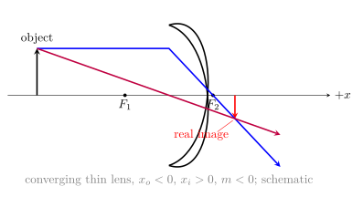
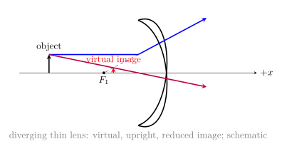
会聚薄透镜的三条主光线:平行入射后过像方焦点;过物方焦点后平行;过 optical center 在薄透镜近似中不偏折。发散透镜的平行入射光出射后发散,其反向延长通过物方虚焦点。
Knowledge 3 — Lens-maker equation and optical power / 透镜制造者公式与光焦度
Knowledge ID: P05-U02-L03-K03
由上一节两表面相加可直接读出薄透镜制造者公式:
\[\boxed{\frac1f= \left(\frac{n_\ell}{n_m}-1\right) \left(\frac1{R_1}-\frac1{R_2}\right)}.\]
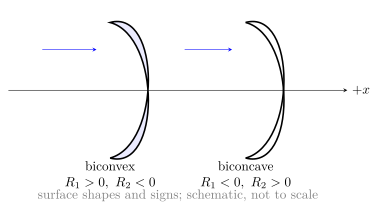
曲率半径由曲率中心位置定号。对左入射的双凸透镜,第一面中心在右,\(R_1>0\);第二面中心在左,\(R_2<0\),所以通常 \(f>0\)。双凹则相反。
光焦度定义为
\[\boxed{\Phi=\frac1f},\]
当 \(f\) 用 m 时单位是 diopter:\(1\,\mathrm D=1\,\mathrm{m^{-1}}\)。浸入液体后,真正起作用的是相对折射率 \(n_\ell/n_m\);若 \(n_m\) 接近 \(n_\ell\),透镜光焦度减小。若外界折射率高于透镜材料,原来会聚的形状甚至可能变为发散。
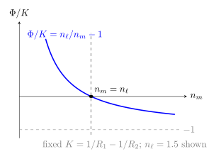
该式忽略中心厚度。厚透镜需保留两面间距,焦距应相对 principal planes 定义;仅从几何中心测量会产生系统误差。
Knowledge 4 — Multiple lenses and equivalent systems / 多透镜与等效系统
Knowledge ID: P05-U02-L03-K04
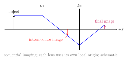
逐元件追迹:中间像就是下一步的物
设第 1、2 透镜的全局位置为 \(X_1,X_2\)。物的全局坐标为 \(X_O\)。对第一透镜使用局部物坐标
\[x_{o1}=X_O-X_1,\]
求得 \(x_{i1}\) 后,中间像全局位置为
\[X_{I1}=X_1+x_{i1}.\]
第二透镜看到的局部物坐标是
\[x_{o2}=X_{I1}-X_2.\]
若 \(x_{o2}<0\),中间像在第二透镜左侧,是实物;若 \(x_{o2}>0\),进入第二透镜的光已朝右侧某点会聚,该点是第二透镜的 virtual object。最终总放大率为 \(m=m_2m_1\)。
两片薄透镜接触时 \(d=0\),光焦度相加:
\[\Phi_{\mathrm{eq}}=\Phi_1+\Phi_2.\]
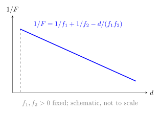
若在同一介质中相隔 \(d\),一阶等效焦度为
\[\boxed{\frac1F=\frac1{f_1}+\frac1{f_2}-\frac{d}{f_1f_2}}.\]
此 \(F\) 是系统 effective focal length;front/back focal distances 还取决于 principal-plane 位移,通常不都等于 \(F\)。
Knowledge 5 — ABCD ray-transfer matrices / ABCD 光线传递矩阵
Knowledge ID: P05-U02-L03-K05
光线状态与基本矩阵
近轴光线在某平面由高度 \(y\) 和小角斜率 \(\theta\) 决定:
\[\mathbf r= \begin{pmatrix}y\\ \theta\end{pmatrix}.\]
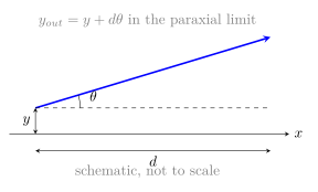
在均匀介质中向右传播距离 \(d\):
\[y_{\mathrm out}=y_{\mathrm in}+d\theta_{\mathrm in}, \qquad \theta_{\mathrm out}=\theta_{\mathrm in},\]
\[\boxed{P(d)= \begin{pmatrix}1&d\\0&1\end{pmatrix}}.\]
通过焦距 \(f\) 的理想薄透镜:
\[y_{\mathrm out}=y_{\mathrm in}, \qquad \theta_{\mathrm out}=\theta_{\mathrm in}-\frac{y_{\mathrm in}}f,\]
\[\boxed{L(f)= \begin{pmatrix}1&0\\-1/f&1\end{pmatrix}}.\]
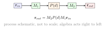
顺序:右边矩阵先作用
若光依次遇到 \(M_1\)、传播、再遇到 \(M_2\),则
\[\mathbf r_{\mathrm out} =M_2P(d)M_1\mathbf r_{\mathrm in}.\]
一般系统写成
\[M=\begin{pmatrix}A&B\\C&D\end{pmatrix}, \qquad \mathbf r_{\mathrm out}=M\mathbf r_{\mathrm in}.\]
同一输入物平面上的一点会发出不同 \(\theta_{\mathrm in}\) 的光线。若输出平面要把它们聚到同一 \(y_{\mathrm out}\),必须消去角度依赖,因此 imaging condition 是
\[\boxed{B=0}.\]
对于上述无损同介质基本矩阵,\(\det M=AD-BC=1\),可作为乘法自检。
若系统跨越不同折射率,直接用 \((y,\theta)\) 会使界面矩阵行列式含折射率比。改用 reduced angle \((y,n\theta)\) 可保持许多无损系统的 symplectic form;必须先声明选用哪一种 ray vector,不能混合表格。
Worked Examples / 完整例题
Worked Example 1 — Imaging by one spherical refracting surface
空气 \(n_1=1.00\) 中的物点位于球面顶点左侧 \(0.300\,\mathrm m\);右侧玻璃 \(n_2=1.50\),曲率中心在右侧 \(0.100\,\mathrm m\)。求像坐标与放大率。
研究对象: 单个球面折射界面。
参考系/系统: 界面静止,光从左向右。
坐标: \(x_o=-0.300\,\mathrm m\),\(R=+0.100\,\mathrm m\)。
模型: 近轴、透明、各向同性。
\[\frac{1.50}{x_i}-\frac{1.00}{-0.300} =\frac{1.50-1.00}{0.100}=5.00\,\mathrm{m^{-1}}.\]
\[\frac{1.50}{x_i}=1.667\,\mathrm{m^{-1}}, \qquad \boxed{x_i=+0.900\,\mathrm m}.\]
\[m=\frac{n_1x_i}{n_2x_o} =\frac{(1.00)(0.900)}{(1.50)(-0.300)}=-2.00.\]
检查: \(x_i>0\) 为玻璃内实像;\(m<0\) 倒立;每项量纲均为 \(\mathrm{m^{-1}}\)。三位有效数字。
Worked Example 2 — Converging thin lens
会聚薄透镜 \(f=+0.120\,\mathrm m\),高 \(3.00\,\mathrm{cm}\) 的物体位于 \(x_o=-0.300\,\mathrm m\)。求像。
研究对象: 同一空气中的理想薄透镜。
参考系/系统: 透镜静止,光左向右。
坐标: 透镜平面为 \(x=0\),高度向上为正。
模型: 近轴、薄透镜。
\[\frac1{x_i}=\frac1f+\frac1{x_o} =\frac1{0.120}+\frac1{-0.300} =5.000\,\mathrm{m^{-1}},\]
\[x_i=+0.200\,\mathrm m, \qquad m=\frac{0.200}{-0.300}=-0.667.\]
\[y_i=(-0.667)(3.00\,\mathrm{cm})=-2.00\,\mathrm{cm}.\]
答案: 透镜右侧 \(0.200\,\mathrm m\) 的倒立、缩小实像。
检查: \(x_i>f\) 且 \(x_o<-f\);单位、方向与主光线一致。三位有效数字。
Worked Example 3 — Same lens shape in air and water
对称双凸薄透镜 \(n_\ell=1.600\),\(R_1=+0.200\,\mathrm m\)、\(R_2=-0.200\,\mathrm m\)。分别求在空气 \(n_m=1.000\) 与水 \(n_m=1.333\) 中的光焦度和焦距。
研究对象: 固定曲率的薄透镜。
参考系/系统: 外介质均匀且两侧相同。
坐标: 曲率中心在右为正。
模型: 薄透镜、近轴、忽略色散。
曲率因子
\[\frac1{R_1}-\frac1{R_2}=5.00-(-5.00)=10.0\,\mathrm{m^{-1}}.\]
空气中
\[\Phi_{\mathrm{air}}=(1.600-1)(10.0)=6.00\,\mathrm D, \qquad f_{\mathrm{air}}=0.167\,\mathrm m.\]
水中
\[\Phi_{\mathrm{water}}=\left(\frac{1.600}{1.333}-1\right)(10.0) =2.00\,\mathrm D,\]
\[f_{\mathrm{water}}=0.499\,\mathrm m.\]
检查: 水使相对折射率更接近 1,故光焦度下降、焦距增大;\(\mathrm D=\mathrm{m^{-1}}\)。输入数据支持约三位有效数字。
Worked Example 4 — Two separated lenses by ABCD matrices
空气中先遇到 \(f_1=+0.100\,\mathrm m\) 的薄透镜,传播 \(d=0.0500\,\mathrm m\),再遇到 \(f_2=+0.200\,\mathrm m\) 的薄透镜。求总矩阵、effective focal length,以及平行入射光从第二透镜后传播多远聚焦。
研究对象: 两薄透镜与中间自由空间。
参考系/系统: 同一静止空气,光从左向右。
坐标: ray vector 为 \((y,\theta)^{\mathsf T}\)。
模型: 近轴、无厚度、无损。
遇到顺序为 \(L_1\to P(d)\to L_2\),所以
\[M=L(f_2)P(d)L(f_1).\]
\[M= \begin{pmatrix}1&0\\-5&1\end{pmatrix} \begin{pmatrix}1&0.0500\\0&1\end{pmatrix} \begin{pmatrix}1&0\\-10&1\end{pmatrix} =\begin{pmatrix}0.500&0.0500\\-12.5&0.750\end{pmatrix}.\]
\[F=-\frac1C=0.0800\,\mathrm m.\]
平行输入 \(\theta_{in}=0\) 后,在第二透镜处 \(y'=Ay\)、\(\theta'=Cy\)。再传播 \(\ell\) 聚焦需 \(y'+\ell\theta'=0\):
\[\ell=-\frac AC=-\frac{0.500}{-12.5}=0.0400\,\mathrm m.\]
检查: \(\det M=(0.500)(0.750)-(0.0500)(-12.5)=1.000\);\(F\) 与 \(1/F=1/f_1+1/f_2-d/(f_1f_2)=12.5\,\mathrm{m^{-1}}\) 一致。三位有效数字。
Lesson synthesis / 本课综合
一阶几何光学的主线是:以笛卡尔坐标写单球面折射 → 把两面相加并取薄透镜极限 → 用 lens-maker equation 把焦距连接到材料与曲率 → 将中间像作为下一元件的物逐步追迹 → 最后把每个线性步骤写成 ABCD 矩阵。坐标符号与矩阵顺序都必须在计算前声明,并用主光线、量纲、\(\det M\) 和极限情况复核。
Formula-and-decision table / 公式与决策表
| Need | Formula | Conditions | Main caution |
|---|---|---|---|
| one refracting surface | \(n_2/x_i-n_1/x_o=(n_2-n_1)/R\) | spherical, paraxial | \(R\) is center coordinate |
| thin-lens image | \(1/x_i-1/x_o=1/f\) | same external medium, thin lens | differs from mirror equation |
| lens magnification | \(m=x_i/x_o\) | thin lens, paraxial | sign gives orientation |
| lens construction | \(1/f=(n_\ell/n_m-1)(1/R_1-1/R_2)\) | thin lens | surrounding medium matters |
| two separated lenses | \(1/F=1/f_1+1/f_2-d/(f_1f_2)\) | same medium, paraxial | \(F\) is not every focal distance |
| free propagation | \(P(d)=\begin{pmatrix}1&d\\0&1\end{pmatrix}\) | ray vector \((y,\theta)\) | \(\theta\) in radians |
| thin lens matrix | \(L(f)=\begin{pmatrix}1&0\\-1/f&1\end{pmatrix}\) | ideal thin lens | total product is reverse encounter order |
| plane-to-plane imaging | \(B=0\) | \(M\) maps chosen input plane to output plane | depends on selected planes |
Model boundaries / 模型边界
- 所有 Gaussian imaging equations 都要求近轴;high-NA systems 必须做精确 ray tracing 或 wave optics。
- 薄透镜忽略中心厚度与 principal-plane separation;厚透镜不能从几何中心套同一公式。
- Lens-maker equation 中 \(n\) 随波长变化,因此真实焦距也有 chromatic dispersion。
- 多透镜逐步成像在每一步都必须重置局部原点;把全局位置误当局部距离会制造符号错误。
- ABCD matrices 描述一阶 ray geometry,不包含 aperture clipping、diffraction、aberration、polarization 或 Fresnel loss。
- 使用 \((y,\theta)\) 与 \((y,n\theta)\) 会得到不同界面矩阵;只有在同一向量定义中组合才合法。
Misconception clinic / 误区诊所
- “双凸透镜一定会聚。” 在通常空气中是,但光焦度取决于 \(n_\ell/n_m\);浸入更高折射率介质可改变甚至反转符号。
- “虚物不是真实计算对象。” 虚物表示进入下一元件的光已朝其出射侧某点会聚,是完全明确的 incoming ray state。
- “两片透镜的焦度总可直接相加。” 只有接触时如此;分离 \(d\) 带来 \(-d/(f_1f_2)\) 项和主平面位移。
- “矩阵按光线遇到顺序从左向右相乘。” 列向量右乘约定下,先遇到的矩阵写在最右边。
- “\(F=80\,\mathrm{mm}\) 就表示最后一片后焦距也是 \(80\,\mathrm{mm}\)。” 对分离系统,effective focal length 与 back focal distance 一般不同。
Practice and retrieval / 练习与提取
- K01 计算: 平面界面 \(R\to\infty\),物在玻璃 \(n_1=1.50\) 中 \(x_o=-0.120\,\mathrm m\),观察侧为空气 \(n_2=1.00\)。求像坐标。
Answer
\[\frac{1.00}{x_i}=\frac{1.50}{-0.120}, \qquad x_i=-0.0800\,\mathrm m.\] 像与物在同一侧,是较浅的虚像。
- K01 符号: 球面曲率中心在顶点左侧 \(0.250\,\mathrm m\),本课 \(R\) 是多少?
Answer
\(R=-0.250\,\mathrm m\);符号由中心坐标决定,与表面被口头称作凸或凹无关。
- K02 计算: 发散透镜 \(f=-0.150\,\mathrm m\),实物 \(x_o=-0.600\,\mathrm m\)。求 \(x_i,m\)。
Answer
\[\frac1{x_i}=\frac1{-0.150}+\frac1{-0.600}=-8.333\,\mathrm{m^{-1}},\] \[x_i=-0.120\,\mathrm m, \qquad m=\frac{-0.120}{-0.600}=+0.200.\] 是物方的正立缩小虚像。
- K02 极限: 会聚透镜的实物恰在物方焦点时,出射光怎样?
Answer
\(x_o=-f\) 使 \(1/x_i=1/f+1/x_o=0\),故像在无穷远,出射光平行。
- K03 计算: 空气中 plano-convex 薄透镜 \(n=1.50\),\(R_1=+0.200\,\mathrm m\)、\(R_2\to\infty\)。求 \(\Phi,f\)。
Answer
\[\Phi=(1.50-1)\left(\frac1{0.200}-0\right)=2.50\,\mathrm D,\] \[f=0.400\,\mathrm m.\]
- K03 概念: 同一玻璃透镜浸入与玻璃折射率完全相同的液体中,一阶光焦度是多少?
Answer
\(n_\ell/n_m=1\),故 lens-maker equation 给 \(\Phi=0\);界面没有折射率反差,透镜形状不再聚焦。
- K04 计算: 两片接触薄透镜光焦度分别为 \(+4.00\,\mathrm D\) 与 \(-1.50\,\mathrm D\)。求等效焦距。
Answer
\[\Phi_{eq}=2.50\,\mathrm D, \qquad F=1/\Phi_{eq}=0.400\,\mathrm m.\]
- K04 虚物: 第 1 透镜的中间像全局位置 \(X_{I1}=0.40\,\mathrm m\),第 2 透镜在 \(X_2=0.30\,\mathrm m\)。对第 2 透镜,\(x_{o2}\) 与物的类型是什么?
Answer
\[x_{o2}=X_{I1}-X_2=+0.10\,\mathrm m.\] 入射光正在朝第二透镜右侧的点会聚,所以这是 virtual object。
- K05 矩阵: 写出光依次传播 \(d_1\)、过透镜 \(f\)、再传播 \(d_2\) 的总矩阵顺序。
Answer
\[M=P(d_2)L(f)P(d_1).\] 最先发生的 \(P(d_1)\) 写在最右边。
- K05 成像条件: 若 \(M=\begin{pmatrix}A&B\\C&D\end{pmatrix}\) 把物平面映到候选像平面,为什么 \(B=0\) 表示成像?
Answer
因 \(y_{out}=Ay_{in}+B\theta_{in}\)。同一物点固定 \(y_{in}\) 却发出不同 \(\theta_{in}\);只有 \(B=0\) 时所有这些光线到达同一 \(y_{out}=Ay_{in}\)。
Exit ticket / 离堂检核
- 从两个球面折射式消去中间像,重建薄透镜公式和 lens-maker equation,并逐一说明 \(R_1,R_2\) 的符号。
- 给定三个按空间顺序排列的元件,写出总 ABCD 矩阵,解释为何最先遇到的元件在最右,并给出两种独立自检。
References and source notes / 参考资料与来源说明
Source-to-content map
| Source | Used for | Knowledge ID / section | Model boundary or convention |
|---|---|---|---|
| OpenStax University Physics Vol. 3, 2.3 Images Formed by Refraction | spherical-interface imaging and apparent/real image structure | K01 | source distance signs converted to the stated Cartesian coordinates |
| OpenStax University Physics Vol. 3, 2.4 Thin Lenses | thin-lens derivation, ray rules, lens-maker equation, magnification | K02–K03 | thin and paraxial approximation |
| MIT 6.161, Geometric Optics notes, Section 2.2 Ray Transfer Matrix Formalism | \((y,\theta)\) matrices for free space and thin lenses | K05 | same ray-vector convention must be retained |
| UC San Diego Physics 4L, Introduction to Optical Design with the ABCD Matrix Technique | interface/propagation logic, matrix composition and optical design checks | K04–K05 | paraxial rays and forward propagation |
| MIT OCW 2.71, Lecture 4: Sign Conventions; Thin Lenses; Real and Virtual Images | sign discipline, power, real/virtual imaging, matrix approach | K01–K05 | conventions differ across texts and must not be mixed |
| Feynman Lectures Vol. I, Ch. 27: Geometrical Optics | successive surfaces, principal-plane concept and paraxial boundary | K01–K04 | thin lens is a limiting case of a general system |
资料和链接实际打开核对日期:2026-08-28。所有图均按本文坐标与方程原创绘制;例题与练习独立复算。
复习与拓展
- Reflection and Refraction:Snell 定律与平面界面。
- Mirrors:比较反射与折射的符号、公式和放大率。
- The Eye and Cameras:把薄透镜、光焦度与 sensor/retina plane 相连。
- Magnifiers, Microscopes, and Telescopes:多元件角放大与焦点配置。
- Gaussian optics:把 ABCD 矩阵作用扩展到 complex beam parameter \(q\)。