多电子原子 · Many-Electron Atoms

Learning objectives / 学习目标

完成本课后，你应能：

写出 $$nl^N$$ configuration，区分 shell、subshell、orbital 与 spin-orbital，并做容量计数。
从多电子 Hamiltonian 解释 screening、penetration 与 effective nuclear charge 的模型性质。
用 Pauli principle 和 Aufbau/Madelung heuristic 生成基态候选，并识别常见例外与离子化顺序。
对给定 open shell 运用 Hund's rules 确定最可能的 ground term，同时明确规则成立条件。
在 electrostatic interaction 与 spin–orbit interaction 的相对强弱之间选择 LS 或 jj coupling，并写出 term symbols。
用微观态计数、宇称和总简并度检查 configuration/term 推理。

Prerequisites / 先修知识

Hydrogenic Atoms and Corrections： $$nL_j$$ 与 spin–orbit。
Identical Particles：fermionic antisymmetry、Pauli principle、Slater determinants。
Addition of Angular Momentum：三角规则与 Clebsch–Gordan decomposition。

Scope and conventions / 范围与约定

研究孤立中性原子或离子，核固定于原点；能量按 nonrelativistic Coulomb Hamiltonian 加 spin–orbit 的层级组织。
configuration 是 occupied one-electron orbitals 的标签，不是精确 many-body eigenfunction；同一 configuration 可产生多个 terms。
“ $Z_{\rm eff}$ ”只作为指定 orbital/observable 下的模型参数，不能给整个原子一个唯一常数。
Aufbau/Madelung order 是经验性 ground-state heuristic，不是普适定理；transition metals、lanthanides、ions 需依据能量与实测数据。
term symbol 用 $^{2S+1}L_J$ ，odd parity 以 $\mathord{}^\circ$ 或文字 odd 标明；正文用 $\pi=(-1)^{\sum_i\ell_i}$ 避免字体歧义。

Notation and modeling contract / 符号与建模契约

Symbol	Meaning	SI unit
$$N,Z$$	电子数与核电荷数	1
$$nl^q$$	$$nl$$ subshell 占据 $$q$$ 个电子	1
$Z_{\rm eff}$	某 orbital 感受的有效核电荷	1
$\mathbf L=\sum_i\mathbf l_i$	总轨道角动量	$\mathrm{J\,s}$
$\mathbf S=\sum_i\mathbf s_i$	总自旋	$\mathrm{J\,s}$
$\mathbf J=\mathbf L+\mathbf S$	总电子角动量	$\mathrm{J\,s}$
$g=2(2\ell+1)$	$$nl$$ subshell 最大电子数	1

1. Electron configurations and shell structure / 电子组态与壳层结构

Knowledge ID: P08-U01-L02-K01

同一 $$n$$ 属于 shell；同一 $n,\ell$ 属于 subshell；给定 $n,\ell,m_\ell$ 是 spatial orbital，再配 $m_s=\pm1/2$ 得 spin-orbital。于是

$N_{nl}=2(2\ell+1), \qquad N_n=2\sum_{\ell=0}^{n-1}(2\ell+1)=2n^2.$

例如 oxygen 的 ground configuration 写作 $$1s^22s^22p^4$$ 或 $[\mathrm{He}]2s^22p^4$ 。closed subshell 的 $$L=S=0$$ ，因而在 term analysis 中常作为 inert core，但它仍贡献屏蔽、总能量与相关效应。

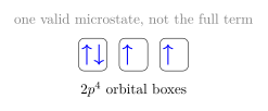
Many-Electron Atoms — 1. Electron configurations and shell structure / 电子组态与壳层结构（图 1） — 图 11. Electron configurations and shell structure / 电子组态与壳层结构

图 1 是 $$2p^4$$ 的一个 microstate；三个盒子表示 $m_\ell=-1,0,1$ ，箭头是 spin projection，不是电子经典转向。

Many-Electron Atoms — 1. Electron configurations and shell structure / 电子组态与壳层结构（图 2） — 图 21. Electron configurations and shell structure / 电子组态与壳层结构

图 2 把常被混用的四级结构区分开，并给出逐层 capacity。

2. Shielding and effective nuclear charge / 屏蔽与有效核电荷

Knowledge ID: P08-U01-L02-K02

多电子 Hamiltonian 含不可分离项

$H=\sum_i\left(\frac{p_i^2}{2m_e}-\frac{Ze^2}{4\pi\epsilon_0r_i}\right) +\sum_{i<j}\frac{e^2}{4\pi\epsilon_0r_{ij}}.$

central-field approximation 把其他电子的平均作用写入 $V_{\rm eff}(r)$ 。远离核时，内层电子部分抵消核电荷；但 penetration 较强的 $$s$$ orbital 在小 $$r$$ 更常采样未屏蔽核，因此同一 $$n$$ 中通常 $$s$$ 比 $$p,d$$ 更低能。粗略 hydrogenic estimate 为

$E_{n\ell}\sim-13.6\,\mathrm{eV}\frac{Z_{\rm eff}^2}{n^2},$

但 $Z_{\rm eff}$ 依赖 $n,\ell$ 与所用方法，不能从单一观测无歧义推广到所有态。

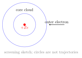
Many-Electron Atoms — 2. Shielding and effective nuclear charge / 屏蔽与有效核电荷（图 3） — 图 32. Shielding and effective nuclear charge / 屏蔽与有效核电荷

图 3 表示外层电子看到核与 core electron cloud 的合成场；轨道云不能用同心经典轨道解释。

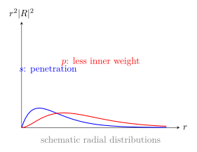
Many-Electron Atoms — 2. Shielding and effective nuclear charge / 屏蔽与有效核电荷（图 4） — 图 42. Shielding and effective nuclear charge / 屏蔽与有效核电荷

图 4 只比较 inner-region weight 的趋势；具体节点与峰位置依赖 orbital，不按比例。

3. Pauli principle and Aufbau ordering / 泡利原理与构造顺序

Knowledge ID: P08-U01-L02-K03

fermionic antisymmetry 要求任意两个电子不能占同一 spin-orbital，即同一原子中不能有完全相同的四个 one-electron quantum numbers。它严格给出“每 orbital 最多两电子且自旋相反”，但不决定不同 subshell 的能量次序。

Aufbau 候选常按 Madelung rule：先小 $n+\ell$ ，相同则先小 $$n$$ 。这是 mean-field energy pattern 的经验压缩； $$4s/3d$$ 、 $$5s/4d$$ 等能量接近，exchange、correlation 与 ionization 会改变次序。写 transition-metal ion 时通常先移去最大 $$n$$ 的 $$s$$ electrons。

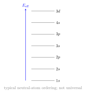
Many-Electron Atoms — 3. Pauli principle and Aufbau ordering / 泡利原理与构造顺序（图 5） — 图 53. Pauli principle and Aufbau ordering / 泡利原理与构造顺序

图 5 是常用 Aufbau ladder，但刻意标为 typical；能级会随 $$Z$$ 、charge state 与 configuration 重排。

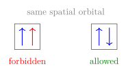
Many-Electron Atoms — 3. Pauli principle and Aufbau ordering / 泡利原理与构造顺序（图 6） — 图 63. Pauli principle and Aufbau ordering / 泡利原理与构造顺序

图 6 对比相同与相反 spin projections；两箭头只是 basis labels，Pauli 的根源是 total wavefunction antisymmetry。

4. Hund's rules / 洪特规则

Knowledge ID: P08-U01-L02-K04

对给定 configuration 且 LS coupling 良好，ground term 的经验顺序为：

最大化 $$S$$ （最大 multiplicity $$2S+1$$ ）；
在该 $$S$$ 下最大化 $$L$$ ；
少于半满 shell 取最小 $J=\lvert L-S\rvert$ ，多于半满取最大 $$J=L+S$$ ；半满常 $$L=0$$ 。

前两条源于 exchange 与电子回避带来的 Coulomb energy lowering，不应误说成“平行自旋直接吸引”。第三条反映 spin–orbit energy 与 shell filling；强 configuration mixing 或 jj regime 下需直接 diagonalize。

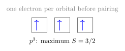
Many-Electron Atoms — 4. Hund's rules / 洪特规则（图 7） — 图 74. Hund's rules / 洪特规则

图 7 展示 half-filled $$p^3$$ 的最大自旋 microstate；它提示 $$^4S$$ ground term，但 term 仍是许多 microstates 的线性组合。

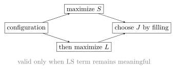
Many-Electron Atoms — 4. Hund's rules / 洪特规则（图 8） — 图 84. Hund's rules / 洪特规则

图 8 是 Hund workflow；它不是按 orbital 箭头机械背诵的替代品，必须先确认 configuration 与 coupling regime。

5. LS and jj coupling / LS 与 jj 耦合

Knowledge ID: P08-U01-L02-K05

轻原子通常 electron–electron electrostatic splitting 大于各电子 spin–orbit splitting，先合成

$\mathbf L=\sum_i\mathbf l_i, \qquad \mathbf S=\sum_i\mathbf s_i, \qquad \mathbf J=\mathbf L+\mathbf S,$

得到 $^{2S+1}L_J$ ，称 LS 或 Russell–Saunders coupling。重原子中单电子 spin–orbit 较强，可先形成 $\mathbf j_i=\mathbf l_i+\mathbf s_i$ ，再 $\mathbf J=\sum_i\mathbf j_i$ ，称 jj coupling。真实原子常在 intermediate coupling，标签表示 dominant component 而非精确守恒量。

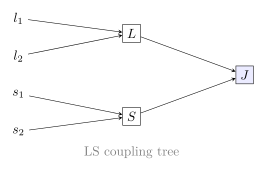
Many-Electron Atoms — 5. LS and jj coupling / LS 与 jj 耦合（图 9） — 图 95. LS and jj coupling / LS 与 jj 耦合

图 9 明确 LS coupling 的运算顺序；线条是 angular-momentum coupling tree，不是力或时间演化。

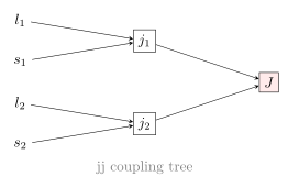
Many-Electron Atoms — 5. LS and jj coupling / LS 与 jj 耦合（图 10） — 图 105. LS and jj coupling / LS 与 jj 耦合

图 10 与图 9 使用同一输入角动量却改变先后顺序；两种 basis spans 相同，差别在何种 interaction 使哪个 basis 接近 diagonal。

Worked Examples / 完整例题

Worked Example 1 — subshell 与 shell capacity

问题与系统。 研究 isolated atom 的 $$n=4$$ shell；只做 spin-orbital state counting，不讨论能量。

允许 $\ell=0,1,2,3$ ，各容量 $2(2\ell+1)=2,6,10,14$ ，因此

$\[N_4=2+6+10+14=32=2n^2.\]$

检查。 计数无量纲；每个 spatial orbital 的两自旋态已计入。这个 32 不是中性原子“必然占据数”，只是 shell 最大容量。

Worked Example 2 — 用 hydrogenic estimate 比较屏蔽

已知与模型。 两个同 $$n=3$$ orbital 拟合得 $Z_{\rm eff}(3s)=4.0$ 、 $Z_{\rm eff}(3d)=2.8$ 。研究 central-field one-electron energies，忽略 correlation。

$E_{3s}\approx-13.6\frac{4.0^2}{9}=-24.2\,\mathrm{eV},$

$E_{3d}\approx-13.6\frac{2.8^2}{9}=-11.8\,\mathrm{eV}.$

检查与解释。 更 penetrative 的 $$3s$$ 看到更大 $Z_{\rm eff}$ ，binding 更强。eV 来自 energy scale， $Z_{\rm eff}^2/n^2$ 无量纲。这只是 state-dependent fit，不能把差值当精确 excitation energy。

Worked Example 3 — carbon $$2p^2$$ ground term

系统与耦合。 neutral carbon open shell $$2p^2$$ ，closed core 忽略角动量；轻原子采用 LS coupling。Hund 1 最大 $$S=1$$ ，Hund 2 在此取最大允许 $$L=1$$ ，故 term 为 $$^3P_J$$ 。少于半满 $$p$$ shell，Hund 3 取最小 $J=\lvert L-S\rvert=0$ ，ground level $$^3P_0$$ 。

检查。 $$J=0,1,2$$ 均满足三角规则；term magnetic states 总数 $1+3+5=9=(2S+1)(2L+1)=3\times3$ 。结论依赖 LS 与 Hund 条件。

Worked Example 4 — 识别 coupling regime

已知。 某 configuration 的 electrostatic term separation 约 $1.2\,\mathrm{eV}$ ，single-electron spin–orbit splitting 约 $0.03\,\mathrm{eV}$ 。另一重原子 configuration 两者分别约 $0.20\,\mathrm{eV}$ 与 $0.35\,\mathrm{eV}$ 。

模型判断。 第一例比值 $0.03/1.2=0.025\ll1$ ，先形成 $$L,S$$ ，LS labels 稳健。第二例比值 $$0.35/0.20=1.75$$ ，spin–orbit 不再是小扰动，jj 或 intermediate coupling 更合适。

检查与解释。 比值无量纲；这只是 regime diagnostic，真实 Hamiltonian 仍需在完整 basis diagonalize，不能仅按阈值自动选择唯一标签。

Lesson synthesis / 全课综合

多电子原子从“精确不可分离”变为“可标记”的流程是：选择 antisymmetrized spin-orbitals → 以 mean central field 建 configuration → 用 screening/penetration 理解 orbital order → 用 Pauli 排除非法占据 → 在适用时用 Hund 找最低 term → 比较 electrostatic 与 spin–orbit 能标后选 LS、jj 或 intermediate basis → 用 NIST level data 校验。

Formula-and-decision table / 公式与决策表

Need	Formula/rule	Use when	Limitation
subshell capacity	$2(2\ell+1)$	state counting	not occupancy prediction
shell capacity	$$2n^2$$	hydrogenic label set	energies not degenerate in many-electron atoms
Hamiltonian	$\sum_i h_i+\sum_{i<j}e^2/(4\pi\epsilon_0r_{ij})$	define full problem	not separable
rough binding	$-13.6Z_{\rm eff}^2/n^2$ eV	qualitative central field	$Z_{\rm eff}$ state dependent
LS label	$^{2S+1}L_J$	electrostatic $\gg$ spin–orbit	intermediate coupling common
parity	$(-1)^{\sum_i\ell_i}$	configuration parity	configuration mixing only within same parity
Hund rules	max $$S$$ , max $$L$$ , then $$J$$	ground term in good LS shell	not universal theorem

Model boundaries / 模型边界

Independent-particle orbitals omit dynamical correlation.
$Z_{\rm eff}$ is observable/model dependent, not an operator eigenvalue common to all electrons.
Madelung order has known exceptions and changes under ionization.
Hund rules apply to a specified configuration and adequate LS coupling.
Closed shell has $$L=S=0$$ but is not physically absent.
LS and jj are basis limits; intermediate coupling requires diagonalization and mixed labels.

Misconception clinic / 误区诊所

“shell、subshell、orbital 是同义词。” 它们依次固定 $$n$$ 、 $(n,\ell)$ 、 $(n,\ell,m_\ell)$ 。
“屏蔽等于内层电子精确抵消若干个质子。” 量子概率云与 penetration 使有效场随 $$r$$ 和 orbital 改变。
“Aufbau 是 Pauli principle 的推论。” Pauli 限制占据；能量次序来自 Hamiltonian 与相互作用。
“Hund 说平行自旋彼此吸引。” lowering 源于 antisymmetry 引起的空间回避与 exchange integral。
“写出 configuration 就确定唯一能级。” 一个 configuration 可分裂为多个 $$L,S,J$$ terms。
“重原子一定是纯 jj。” 许多重原子仍处 intermediate coupling，需看能标和数据。

Practice and retrieval / 练习与提取

K01： 求 $$4f$$ subshell 与 $$n=5$$ shell 的最大电子数。
K01： 区分 $$3p^4$$ 中的 shell、subshell、spatial orbital 和 spin-orbital。
K02： 为什么同一 $$n$$ 中 $$s$$ orbital 通常低于 $$d$$ orbital？
K02： $Z_{\rm eff}=5$ 的 $$n=4$$ 粗略 binding magnitude 是多少？
K03： 判断同一 spatial orbital 内两个 spin-up electrons 是否允许。
K03： 为什么 transition-metal cation 常先失去 $$4s$$ 而非 $$3d$$ electrons？
K04： 用 Hund rules 给出 nitrogen $$2p^3$$ 的 ground term。
K04： Hund rules 为什么不能跨不同 configurations 直接比较？
K05： 写出 $$L=2,S=1$$ 的所有 $$J$$ 与 term labels。
综合： 为陌生重原子谱线提出判断 LS/jj/intermediate coupling 的证据链。

Answers / 答案

$$4f$$ 有 $2(2\cdot3+1)=14$ ； $$n=5$$ shell 有 $$2n^2=50$$ 。
shell 是 $$n=3$$ ；subshell 是 $$3p$$ ；三个 spatial orbitals 对应 $m_\ell=-1,0,1$ ；每个再乘 $m_s=\pm1/2$ 成六个 spin-orbitals。
$$s$$ 在小 $$r$$ 有更强 penetration，平均看到更少屏蔽和更大 nuclear attraction。
$13.6\times25/16=21.25\,\mathrm{eV}$ ；只是模型值。
不允许；四个 one-electron quantum numbers 完全相同，违反 antisymmetry/Pauli。
中性原子填充次序不等于离子化时 orbital energies；形成 $$d$$ occupation 后 $$4s$$ 常更外、更高能。
最大 $$S=3/2$$ ，half-filled 给 $$L=0$$ ，故 $^4S_{3/2}$ 。
它们只排序给定 configuration 内的 terms；configuration average energies 需另算。
$$J=1,2,3$$ ，分别 $$^3D_1,^3D_2,^3D_3$$ 。
比较 electrostatic term separations 与 spin–orbit splittings；检查 observed $$J$$ patterns、Landé intervals、 $$g$$ factors，并以 full-Hamiltonian mixing coefficients/NIST assignments 验证。

Exit ticket / 离堂检验

从 full many-electron Hamiltonian 出发，用四句话连接 screening、Pauli、Hund 与 term symbols。
解释为什么“ $[\mathrm{Ar}]4s^23d^4$ ”既很有用又不是精确 many-body wavefunction。

References and source notes / 参考资料与来源说明

以下来源于 2026-08-30 实际打开核验；正文按统一符号重写，未复制来源图。

Source-to-content map

Source	Used for	Knowledge ID / Section	Model boundary or convention
NIST Atomic States	shell/configuration notation, closed shells	K01–K03	central-field approximation explicit
NIST He/LS	LS hierarchy and $^{2S+1}L_J$	K04–K05	light helium-like regime
NIST Coupling	jj and intermediate labels	K05	labels may denote dominant component
MIT 5.61 Lecture 23	shielding, Slater basis, Hund reasoning	K02–K04	qualitative rules separated from exact diagonalization
OpenStax 8.4	Pauli and periodic configurations	K01, K03	HS intuition extended to UG2
NIST Allowed Terms	equivalent-electron restrictions	K04–K05	tables are validation reference

复习与拓展

Lesson 8.1.3 uses term labels for E1 selection rules and Zeeman/Stark patterns.
Molecular bonding reuses antisymmetry, MO occupancy and bond order.
Solid-state band structure turns many closely spaced orbitals into bands.