
Learning objectives / 学习目标
完成本课后,你应能:
- 由 level populations 与能差区分 absorption、spontaneous emission、stimulated emission 的谱学表现。
- 从 electric-dipole matrix element 推出 parity、\(\Delta J\)、\(\Delta M\) 与 LS-limit rules 的适用层级。
- 用 weak-field Zeeman formula 和 Landé \(g_J\) 计算 sublevel shifts 与 allowed components。
- 判断 nondegenerate quadratic Stark 与 degenerate/near-degenerate linear Stark regimes。
- 区分 natural Lorentzian、Doppler Gaussian、collision Lorentzian 与 Voigt convolution,并计算 FWHM。
- 把 line center、integrated area、peak height 与 instrumental resolution 分开解释。
Prerequisites / 先修知识
- Many-Electron Atoms:configuration、\(^{2S+1}L_J\) 与 coupling。
- Time-Dependent Processes:transition amplitudes、Fermi golden rule、selection rules。
- Coherence and Interferometry:有限相干时间与 linewidth。
Scope and conventions / 范围与约定
- atom 视为稀薄气相中的孤立粒子;实验室系定义 light propagation 与外场轴。
- quantization axis 沿 \(\mathbf B\) 或 \(\mathbf E\);弱场指外场作用小于 fine/hyperfine separation,故 \(J\) 或 \(F\) 仍是 good quantum number。
- 只处理 electric-dipole (E1) 主导跃迁;M1/E2 等“forbidden”线并非严格不可能。
- line profile \(g(\nu)\) 归一化为 \(\int g(\nu)d\nu=1\);FWHM 是全宽而非 half width。
- \(\nu\) 是 Hz,\(\omega=2\pi\nu\) 是 rad s\(^{-1}\);linewidth formulas 不混用二者。
Notation and modeling contract / 符号与建模契约
| Symbol | Meaning | SI unit |
|---|---|---|
| \(\mathbf d=-e\mathbf r\) | electric dipole operator | C m |
| \(J,M\) | 总电子角动量及轴向投影量子数 | 1 |
| \(g_J\) | Landé factor | 1 |
| \(\mu_B\) | Bohr magneton | J T\(^{-1}\) |
| \(\Gamma\) | population decay rate | s\(^{-1}\) |
| \(\Delta\nu\) | FWHM in ordinary frequency | Hz |
| \(\alpha_p\) | static polarizability | C m\(^2\) V\(^{-1}\) |
1. Emission and absorption spectra / 发射与吸收光谱
Knowledge ID: P08-U01-L03-K01
谱线中心首先满足
\[h\nu_0=\lvert E_u-E_l\rvert.\]
absorption 需要 lower state population 和入射 photon;spontaneous emission 需要 upper population;stimulated emission 还与 incident spectral energy density 成正比。测得强度包含 population、transition probability、collection geometry 与 line profile,不能仅由能差决定。
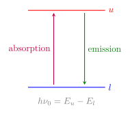
图 1 用同一能差展示吸收与发射;箭头方向编码 energy flow,不代表空间运动。
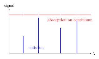
图 2 对比离散 emission peaks 与 continuum 上的 absorption dips;垂直高度由 population 与 apparatus 决定,不等于 energy。
2. Electric-dipole selection rules / 电偶极选择定则
Knowledge ID: P08-U01-L03-K02
E1 transition amplitude 与
\[\langle f\lvert\mathbf d\cdot\boldsymbol\epsilon\rvert i\rangle\]
成正比。由于 \(\mathbf r\) 是 odd-parity rank-1 tensor,严格 angular rules 为 parity change、\(\Delta J=0,\pm1\) 但 \(J=0\not\leftrightarrow J=0\),以及相对 quantization axis 的 \(\Delta M=0,\pm1\)。在良好 LS coupling、configuration mixing 可忽略时还有 \(\Delta S=0\) 与 \(\Delta L=0,\pm1\)(\(L=0\not\leftrightarrow0\))。
“forbidden”表示最低多极矩阵元为零;M1/E2、state mixing、collisions 或外场可使弱线出现。
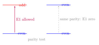
图 3 把 parity change 与 line strength distinction 可视化;虚线只说 E1 matrix element vanish,不说一切辐射绝对禁止。
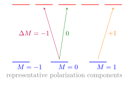
图 4 示意 \(\Delta M\) 与 polarization components;没有画全所有 transitions,不能用线数替代完整 selection-rule enumeration。
3. Zeeman effect / 塞曼效应
Knowledge ID: P08-U01-L03-K03
弱磁场下 \(J,M\) 保持良好,一级位移为
\[\Delta E_{JM}=g_J\mu_BMB,\]
\[g_J=1+\frac{J(J+1)+S(S+1)-L(L+1)}{2J(J+1)}.\]
Landé 分式仅用于 \(J>0\)。对孤立的 \(J=0\) level,一阶 vector magnetic moment 与 \(g_JM\) Zeeman shift 为零;不能把 \(J=0\) 直接代入上式的分母。更高阶 magnetic mixing 仍可能产生二阶位移。
跃迁 component shift 是上、下 level shifts 之差:
\[\Delta\nu=\frac{\mu_BB}{h}(g_uM_u-g_lM_l).\]
strong-field Paschen–Back regime 中 \(L,S\) decouple,不能继续用 weak-field \(g_JM\)。若 hyperfine 先被解析,弱场还应以 \(F,m_F\) 和 \(g_F\) 描述。
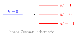
图 5 显示 \(J=1\) level 的等间隔 magnetic sublevels;间隔符号还取决于 \(g_J\) 与 \(B\) 方向。
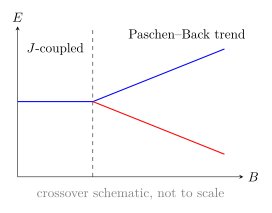
图 6 表示弱场到强场 basis 的 crossover;真实 avoided crossings 与 slopes 需 full Hamiltonian diagonalization。
4. Stark effect / 斯塔克效应
Knowledge ID: P08-U01-L03-K04
uniform electric field \(\mathbf E=E\hat z\) 的 perturbation 是
\[H'=-\mathbf d\cdot\mathbf E=eEz.\]
有 definite parity 的 nondegenerate state 满足 \(\langle z\rangle=0\),一级位移为零;二级位移写为
\[\Delta E^{(2)}=-\frac12\alpha_pE^2,\]
其中 ground-state static polarizability 通常为正。若 opposite-parity states degenerate 或 nearly degenerate,必须在该子空间 diagonalize,可能出现 linear Stark splitting。强场还可能引起 field ionization。
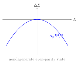
图 7 是 quadratic Stark shift 的偶函数;反转 field 不改变二阶位移。
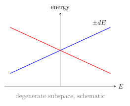
图 8 表示 degenerate manifold 中的 linear branches;直线斜率由 diagonalized dipole eigenvalues 决定。
5. Line broadening and line shapes / 谱线展宽与线型
Knowledge ID: P08-U01-L03-K05
finite lifetime \(\tau=1/\Gamma\) 产生 Lorentzian natural line,ordinary-frequency FWHM
\[\Delta\nu_{\rm nat}=\frac{\Gamma}{2\pi}=\frac{1}{2\pi\tau}.\]
Maxwellian line-of-sight velocity 产生 Gaussian Doppler FWHM
\[\Delta\nu_D=\nu_0\sqrt{\frac{8k_BT\ln2}{mc^2}}.\]
impact collisions 常近似 Lorentzian 并带 pressure shift;Gaussian 与 Lorentzian convolution 是 Voigt profile。instrument response 还需另行 convolution。不同 broadening 若同为 Lorentzian 可加 widths;Gaussian 独立方差可相加,但一般不能把所有 FWHM 直接相加。
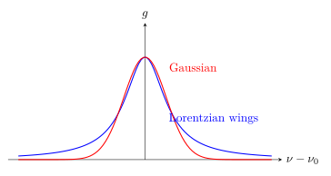
图 9 对比同峰高示意曲线;Lorentzian tails 更重。归一化后峰高会随 width 改变。
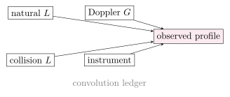
图 10 是 broadening ledger;把 mechanism 分开是从 observed profile 反推温度、压力或 lifetime 的前提。
Worked Examples / 完整例题
Worked Example 1 — absorption line 的能量
已知与系统。 lower/upper energies 差 \(2.10\,\mathrm{eV}\),稀薄冷原子吸收入射光;实验室系,忽略 recoil。
\[\lambda=\frac{hc}{\Delta E}=\frac{1239.841984\,\mathrm{eV\,nm}}{2.10\,\mathrm{eV}}=590\,\mathrm{nm}.\]
检查与解释。 eV 消去留下 nm,三位有效数字。该计算只给 line center;若 lower population 为零或 dipole matrix element 为零,仍不会出现强 absorption。
Worked Example 2 — E1 rule audit
问题。 判断 \(^1S_0\to{}^1P_1^\circ\) 与 \(^3P_0\to{}^1S_0\) 的 E1 性质。
第一条 parity 改变、\(\Delta J=+1\)、\(\Delta S=0\),在 LS limit 强允许。第二条 \(J=0\to0\) 被严格 E1 angular rule 禁止,且 \(\Delta S=1\);即使 spin–orbit mixing 放松 \(\Delta S\),\(0\to0\) E1 仍不允许。
检查。 selection rules 是 matrix-element symmetry audit,不需要 SI 数值;“forbidden”不排除 M1/E2 或 two-photon paths。
Worked Example 3 — Zeeman component shift
已知与模型。 weak field \(B=0.200\,\mathrm T\),某 component 有 \(g_uM_u-g_lM_l=1.50\)。量子化轴沿 \(\mathbf B\)。
取 \(\mu_B/h=13.996245\,\mathrm{GHz\,T^{-1}}\),
\[\Delta\nu=(13.996245)(0.200)(1.50)=4.20\,\mathrm{GHz}.\]
检查与解释。 T\(^{-1}\) 与 T 消去;正号表示相对零场频率上移。必须同时确认 weak-field condition 与 \(\Delta M\) polarization rule。
Worked Example 4 — natural 与 Doppler widths
已知与系统。 \(\lambda_0=500\,\mathrm{nm}\),upper lifetime \(\tau=20.0\,\mathrm{ns}\);质量 \(m=40u\)、\(T=300\,\mathrm K\)。实验室系,热平衡,忽略碰撞。
\[\Delta\nu_{\rm nat}=\frac{1}{2\pi\tau}=7.96\,\mathrm{MHz}.\]
\(\nu_0=c/\lambda_0=5.996\times10^{14}\,\mathrm{Hz}\),\(m=6.642\times10^{-26}\,\mathrm{kg}\),
\[\Delta\nu_D=\nu_0\sqrt{\frac{8k_BT\ln2}{mc^2}} =1.18\,\mathrm{GHz}.\]
检查与解释。 两者单位为 Hz,Doppler 约大 148 倍,room-temperature observed core 主要 Gaussian;窄翼与精密线心仍需 Voigt fit,不能简单丢弃 natural width。
Lesson synthesis / 全课综合
谱学决策顺序:先由 \(E_u-E_l\) 定 center;再由 \(\langle f\lvert\mathbf d\rvert i\rangle\) 与 population 定是否/多强;选外场轴,用 Zeeman/Stark Hamiltonian 求 component centers 与 polarization;最后 convolution natural、thermal、collisional 和 instrumental profiles。中心、面积、峰高、宽度各有不同物理来源。
Formula-and-decision table / 公式与决策表
| Need | Formula | Use when | Main limitation |
|---|---|---|---|
| line center | \(h\nu_0=\lvert E_u-E_l\rvert\) | isolated transition | recoil/shifts omitted |
| E1 strength | \(\lvert\langle f\lvert\mathbf d\cdot\epsilon\rvert i\rangle\rvert^2\) | dipole approximation | higher multipoles omitted |
| weak Zeeman | \(\Delta E=g_J\mu_BMB\) | \(J>0\) and \(J,M\) remain good; \(J=0\) first-order shift is zero | fails in Paschen–Back |
| quadratic Stark | \(-\alpha_pE^2/2\) | nondegenerate parity state | near degeneracy requires matrix diagonalization |
| natural FWHM | \(1/(2\pi\tau)\) | exponential population decay | angular-frequency width differs by \(2\pi\) |
| Doppler FWHM | \(\nu_0\sqrt{8k_BT\ln2/(mc^2)}\) | Maxwellian nonrelativistic gas | bulk flow shifts center |
Model boundaries / 模型边界
- Dipole approximation assumes atomic size much smaller than wavelength.
- LS selection rules weaken under configuration/spin–orbit mixing; parity and \(J\) rules remain symmetry based.
- Weak-field Zeeman fails when field interaction rivals internal splittings.
- Quadratic Stark fails near degeneracy or field ionization.
- Lorentzian/Gaussian profiles assume stationary Markov decay or Maxwellian velocities; speed-dependent collisions can need richer models.
- Apparatus calibration and optical depth can distort line shape and apparent intensity.
Misconception clinic / 误区诊所
- “能差匹配就一定看到强线。” matrix element 与 population 可能使 line absent/weak。
- “forbidden 等于绝不发生。” 它通常只指 E1 leading amplitude 为零。
- “Zeeman splitting 总是等间距三线。” level \(g\) factors、\(M\) ranges、polarization 与 unresolved components 决定 pattern。
- “任何 Stark shift 都线性。” nondegenerate parity eigenstate 的一阶 dipole expectation 通常为零,leading shift 二次。
- “lifetime 越长谱线峰越低。” 固定 integrated area 下,line 越窄峰通常越高;需说明归一化条件。
- “所有 FWHM 可直接相加。” 只有相同 Lorentzian mechanisms 可直接加 widths;Voigt 需 convolution。
Practice and retrieval / 练习与提取
- K01: \(\lambda=400\,\mathrm{nm}\) photon 对应多少 eV?
- K01: 为什么 emission intensity 不能直接等同 Einstein \(A\) coefficient?
- K02: 判断 \(J=1\to J=1\) 与 \(J=0\to J=0\) 的 E1 angular allowance。
- K02: parity 不变的 line 还可能通过哪些 channel 出现?
- K03: \(J=2\) level 在 weak field 中有多少 \(M\) sublevels?
- K03: 何时应从 Zeeman 转用 Paschen–Back description?
- K04: 为什么 definite-parity nondegenerate state 没有 linear Stark shift?
- K05: lifetime \(10\,\mathrm{ns}\) 的 natural FWHM 是多少?
- K05: 把温度提高四倍,Doppler FWHM 变多少倍?
- 综合: 一条谱线变宽且中心随 pressure 移动,提出区分 Doppler 与 collision effects 的实验方案。
Answers / 答案
- \(E=1239.842/400=3.10\,\mathrm{eV}\)。
- measured intensity 还乘 upper population、branching、sample number、geometry、detector response 与 profile integration。
- \(1\to1\) 可允许(仍需 parity change 等);\(0\to0\) E1 严格禁止。
- M1、E2、two-photon、field/configuration mixing 等弱 channel。
- \(2J+1=5\),\(M=-2,-1,0,1,2\)。
- 当 \(\mu_BB\) 与 fine/hyperfine coupling energy 同量级,使原耦合量子数不再良好。
- \(z\) 是 odd-parity operator,故同一 parity state 的 \(\langle z\rangle=0\)。
- \(1/(2\pi\times10\,\mathrm{ns})=15.9\,\mathrm{MHz}\)。
- \(\Delta\nu_D\propto\sqrt T\),故变 2 倍。
- 扫温度与压力:Doppler width 随 \(\sqrt T\) 且近 Gaussian,collision width/shift 随 density/pressure 且近 Lorentzian;做多条件 Voigt global fit,并独立校准 instrument profile。
Exit ticket / 离堂检验
- 对一条有三个 Zeeman components 的线,分别指出 frequency、polarization 与 intensity 由哪些量决定。
- 用“matrix element—population—profile—instrument”四层框架解释为什么同一原子在不同实验中谱图不同。
References and source notes / 参考资料与来源说明
以下来源于 2026-08-30 实际打开核验;正文重组为统一 SI/FWHM convention,图均原创。
- OpenStax University Physics 3 — Atomic Spectra and X-rays
- NIST Atomic Spectroscopy — Spectral Lines and Selection Rules
- NIST Atomic Spectroscopy — Zeeman Effect
- NIST Atomic Spectroscopy — Spectral Line Shapes, Widths, and Shifts
- MIT OCW 5.73 Lecture 24 — Stark and Zeeman Interactions
- NIST Atomic Spectra Database — Lines Form
Source-to-content map
| Source | Used for | Knowledge ID / Section | Model boundary or convention |
|---|---|---|---|
| OpenStax 8.5 | absorption/emission and introductory E1 rules | K01–K02 | extended to term-level UG2 rules |
| NIST Spectral Lines | E1/M1/E2 rules, line strengths | K02 | distinguishes rigorous and LS-only rules |
| NIST Zeeman | \(gM\mu_BB\) and weak-field interpretation | K03 | \(J\) must remain good |
| NIST Line Shapes | Doppler/pressure widths and Gaussian/Lorentz context | K05 | modern precision fits can be more complex |
| MIT 5.73 Lecture 24 | electric/magnetic perturbation operators | K03–K04 | perturbative regimes stated |
| NIST ASD Lines | real wavelengths, probabilities and classifications | K01–K05 | database values benchmark model |
复习与拓展
- Molecular spectroscopy adds rotation, vibration and vibronic band structure.
- Laser physics relates linewidth, saturation and stimulated emission dynamically.
- Precision measurement revisits systematic Stark/Zeeman shifts and Doppler cancellation.