
Learning objectives / 学习目标
学完本课后,你应能:
- 从 species density/velocity 定义 center-of-mass velocity、mass density 与 current,并说明 two-fluid 相对 drift 在 single-fluid model 中保留在哪里;
- 写出 ideal/resistive MHD 的 continuity、momentum、induction、energy/closure 与 \(\nabla\cdot\mathbf B=0\);
- 由 generalized Ohm law 与 Faraday law 推导 induction equation,用 magnetic Reynolds/Lundquist number 判断 advection 与 diffusion;
- 证明 co-moving loop 的 magnetic flux 在 ideal MHD 中守恒,并列出 flux freezing 的模型条件;
- 将 \(\mathbf J\times\mathbf B\) 分解为 magnetic-pressure gradient 与 field-line tension,计算 \(v_A\) 与 plasma beta;
- 解释 reconnection 为什么需要 nonideal electric field,使用 Sweet–Parker scaling 并识别 collisionless/Hall boundary。
Prerequisites / 先修知识
- Kinetic Theory and Vlasov Equation:moments、pressure tensor 与 closure;
- Maxwell equations、vector identities、material derivative 与 continuum conservation;
- Single-Particle Motion:\(\mathbf E\times\mathbf B\) drift 与 magnetization;
- Collisions and Transport:resistivity、collision time 与 anisotropic transport。
Scope and conventions / 范围与约定
- 默认 nonrelativistic, quasineutral electron–singly-ionized plasma;\(\rho\simeq m_in\),但 current \(\mathbf J=en(\mathbf u_i-\mathbf u_e)\) 不设为零。
- SI units;\(\eta\) 表示 electrical resistivity,units \(\Omega\,\mathrm m\);magnetic diffusivity 为 \(\eta_m=\eta/\mu_0\),units \(\mathrm{m^2\,s^{-1}}\)。
- ideal MHD 采用 scalar pressure、negligible electron inertia/Hall/resistivity、large scale \(L\gg d_i,\rho_i\) 与 low frequency \(\omega\ll\omega_{ci}\);每次使用都会复核。
- \(\mathbf B=B\mathbf b\);curvature \(\boldsymbol\kappa=(\mathbf b\cdot\nabla)\mathbf b\) 指向 field-line center of curvature。
- reconnection 图为 two-dimensional schematic;真实 3-D reconnection 的 topology、guide field 与 kinetic dissipation 可更复杂。
Notation and modeling contract / 符号与建模契约
| Symbol | Meaning | SI / convention |
|---|---|---|
| \(\rho\) | mass density | \(\mathrm{kg\,m^{-3}}\) |
| \(\mathbf V\) | center-of-mass velocity | \(\mathrm{m\,s^{-1}}\) |
| \(\mathbf J\) | current density | \(\mathrm{A\,m^{-2}}\) |
| \(p=p_e+p_i\) | total scalar pressure | Pa |
| \(\eta\) | electrical resistivity | \(\Omega\,\mathrm m\) |
| \(\eta_m=\eta/\mu_0\) | magnetic diffusivity | \(\mathrm{m^2\,s^{-1}}\) |
| \(v_A=B/\sqrt{\mu_0\rho}\) | Alfvén speed | \(\mathrm{m\,s^{-1}}\) |
| \(\beta=2\mu_0p/B^2\) | thermal-to-magnetic pressure ratio | dimensionless |
| \(S=\mu_0Lv_A/\eta\) | Lundquist number | dimensionless |
1. Two-fluid and single-fluid descriptions / 双流体与单流体描述
Knowledge ID: P13-U02-L03-K01
1.1 Species equations and composite variables
每个 species 有独立 continuity 与 momentum equation:
\[\frac{\partial n_s}{\partial t}+\nabla\cdot(n_s\mathbf u_s)=0,\]
\[m_sn_s\frac{D_s\mathbf u_s}{Dt} =q_sn_s(\mathbf E+\mathbf u_s\times\mathbf B) -\nabla\cdot\mathbf P_s+\mathbf R_s.\]
两流体描述能保留 electron–ion separation、Hall response、electron pressure 与 different temperatures。定义
\[\rho=m_in_i+m_en_e,\]
\[\mathbf V=\frac{m_in_i\mathbf u_i+m_en_e\mathbf u_e}{\rho}, \qquad \mathbf J=e(n_i\mathbf u_i-n_e\mathbf u_e).\]
quasineutral \(n_i\simeq n_e=n\) 时,\(\mathbf V\simeq\mathbf u_i\) 但 \(\mathbf J=en(\mathbf u_i-\mathbf u_e)\) 可很大;single-fluid 不是强迫两 species 速度相等,而是将 relative velocity 编码为 current。
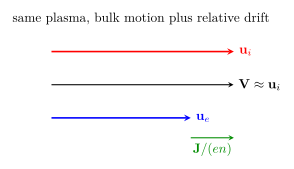
图 1 箭长按所标 schematic velocities;mass weighting 使 bulk arrow 贴近 ion arrow。绿色单向箭头从 electron endpoint 指向 ion endpoint,明确 \(\mathbf J/(en)=\mathbf u_i-\mathbf u_e\) 沿 \(+x\)。
1.2 Generalized Ohm law 作为 model ladder
从 electron momentum equation 可得一种常见 ordering 下的 generalized Ohm law:
\[\mathbf E+\mathbf V\times\mathbf B =\eta\mathbf J +\frac{\mathbf J\times\mathbf B}{en} -\frac{\nabla p_e}{en} +\frac{m_e}{ne^2}\frac{\partial\mathbf J}{\partial t}+\cdots.\]
右侧依次提示 resistive、Hall、electron-pressure 与 electron-inertia corrections。ideal MHD 令右侧近似零;resistive MHD 只保留 \(\eta\mathbf J\)。选择哪一层取决于 \(L/d_i\)、\(\omega/\omega_{ci}\)、collisionality 和 pressure gradients,不能凭装置名称决定。
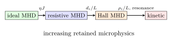
图 2 是 scale hierarchy,不表示右侧模型总比左侧“更好”;合适模型应足够且可验证。
2. Magnetohydrodynamic equations / 磁流体方程
Knowledge ID: P13-U02-L03-K02
ideal MHD 的一组 closed equations 为
\[\frac{\partial\rho}{\partial t}+\nabla\cdot(\rho\mathbf V)=0,\]
\[\rho\left(\frac{\partial\mathbf V}{\partial t}+\mathbf V\cdot\nabla\mathbf V\right) =-\nabla p+\mathbf J\times\mathbf B,\]
\[\mathbf E+\mathbf V\times\mathbf B=0, \qquad \frac{\partial\mathbf B}{\partial t}=-\nabla\times\mathbf E,\]
\[\nabla\times\mathbf B=\mu_0\mathbf J, \qquad \nabla\cdot\mathbf B=0,\]
\[\frac{D}{Dt}\left(\frac{p}{\rho^\Gamma}\right)=0\]
作为 adiabatic scalar-pressure closure。MHD timescale 远慢于 light transit,故 Ampère law 忽略 displacement current。resistive MHD 把 Ohm law 改为 \(\mathbf E+\mathbf V\times\mathbf B=\eta\mathbf J\),从而得到 induction equation:
\[\frac{\partial\mathbf B}{\partial t} =\nabla\times(\mathbf V\times\mathbf B) +\frac{\eta}{\mu_0}\nabla^2\mathbf B\]
(uniform \(\eta\) 且 \(\nabla\cdot\mathbf B=0\))。第一项 advects/stretches field,第二项 diffuses field。
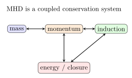
图 3 提醒不能只解 induction equation 而忽略 momentum/closure feedback,除非是明确 kinematic approximation。
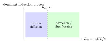
图 4 比较 induction terms;横轴是 regime axis,not to scale。
3. Frozen-in magnetic flux / 磁通冻结
Knowledge ID: P13-U02-L03-K03
对随 fluid velocity \(\mathbf V\) 移动的 closed loop \(C(t)\) 与 spanning surface \(S(t)\):
\[\Phi_B(t)=\int_{S(t)}\mathbf B\cdot d\mathbf S.\]
transport theorem 与 Faraday law 给出
\[\frac{d\Phi_B}{dt} =-\oint_{C(t)}(\mathbf E+\mathbf V\times\mathbf B)\cdot d\boldsymbol\ell.\]
ideal Ohm law 使 integrand 为零,因此
\[\boxed{\frac{d\Phi_B}{dt}=0}.\]
这意味着 material loop 穿过的 magnetic flux conserved,field-line connectivity 在 smooth ideal evolution 中保持。它不表示 field strength 固定:compression 可增大 \(B\),stretching 可改变 direction。更精确地说,flux freezing 要求存在 smooth flux-transport velocity 使 \(\mathbf E+\mathbf V_f\times\mathbf B\) 的 curl-free part 满足 topology preservation。
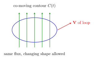
图 5 以 field arrows 穿过 material loop 表示 conserved flux;箭头数量仅为 visual proxy。
4. Magnetic pressure and tension / 磁压与磁张力
Knowledge ID: P13-U02-L03-K04
用 \(\mathbf J=\nabla\times\mathbf B/\mu_0\) 与 \(\nabla\cdot\mathbf B=0\):
\[\mathbf J\times\mathbf B =-\nabla\left(\frac{B^2}{2\mu_0}\right) +\frac{(\mathbf B\cdot\nabla)\mathbf B}{\mu_0}.\]
再写 \(\mathbf B=B\mathbf b\):
\[\frac{(\mathbf B\cdot\nabla)\mathbf B}{\mu_0} =\frac{B}{\mu_0}(\mathbf b\cdot\nabla B)\mathbf b +\frac{B^2}{\mu_0}\boldsymbol\kappa.\]
沿场的 \(B\nabla_\parallel B\) 与 pressure-gradient decomposition 部分抵消,剩余最直观的两项是 perpendicular magnetic-pressure gradient 与 curvature tension \(B^2\boldsymbol\kappa/\mu_0\)。magnetic pressure \(p_B=B^2/(2\mu_0)\) units 为 Pa;tension 像 stretched elastic line,尝试拉直 field。
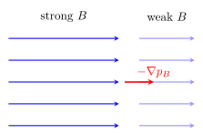
图 6 以 line density 表示 field magnitude;magnetic-pressure force 从强场区指向弱场区。
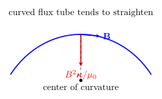
图 7 的 tension 指向 center of curvature;它不是沿 tangent 的 force arrow。
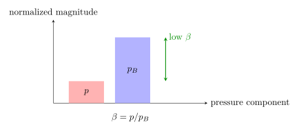
图 8 是 energy/pressure ledger;bar height schematic,公式中的 \(\beta\) 才是 quantitative ratio。
5. Magnetic reconnection / 磁重联
Knowledge ID: P13-U02-L03-K05
ideal flux freezing 禁止 field-line connectivity 改变。reconnection 因此必须有 localized region 满足
\[\mathbf E+\mathbf V\times\mathbf B\ne0.\]
在 resistive MHD 中由 \(\eta\mathbf J\) 支持;在 collisionless diffusion region,Hall term、electron pressure tensor 与 inertia 可支持 nonideal electric field。oppositely directed flux 被带入 current sheet,reconnected field 与 plasma 沿 outflow 喷出,magnetic energy 转为 bulk kinetic、thermal 与 nonthermal particle energy。
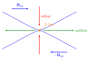
图 9 显示 divergence-free magnetic geometry、inflow/outflow 与 X-point。蓝色曲线只表示穿过 magnetic null 的 separatrix geometry;上、下游短蓝箭头明确标出 antiparallel \(\mathbf B\),红色与绿色箭头才分别是 plasma inflow 和 outflow velocity。
对 steady incompressible Sweet–Parker sheet,length \(L\)、thickness \(\delta\):
\[v_{\rm in}L\sim v_A\delta, \qquad v_{\rm in}B\sim\frac{\eta B}{\mu_0\delta}.\]
所以
\[\frac{\delta}{L}\sim\frac{v_{\rm in}}{v_A}\sim S^{-1/2}, \qquad S=\frac{\mu_0Lv_A}{\eta}.\]
large \(S\) 下 Sweet–Parker 太慢且 sheet 很薄;plasmoid instability、Hall/kinetic effects 或 3-D structure 可改变 rate。
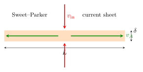
图 10 的 aspect ratio 为 schematic,不按真实 large-\(S\) 比例绘制。
Worked examples / 完整例题
Worked Example 1 — 从 two-fluid velocities 求 \(\mathbf V\) 与 \(\mathbf J\)
已知: uniform hydrogen plasma,\(n_i=n_e=1.00\times10^{19}\ \mathrm{m^{-3}}\),\(\mathbf u_i=1.00\times10^4\hat x\ \mathrm{m\,s^{-1}}\),\(\mathbf u_e=9.00\times10^3\hat x\ \mathrm{m\,s^{-1}}\)。
参考系: laboratory;\(+x\) along both flows。
模型: quasineutral two-fluid definitions。
\[\mathbf J=en(\mathbf u_i-\mathbf u_e) =1.60\times10^3\hat x\ \mathrm{A\,m^{-2}}.\]
\[\mathbf V=\frac{m_i\mathbf u_i+m_e\mathbf u_e}{m_i+m_e} =9.99946\times10^3\hat x\ \mathrm{m\,s^{-1}}.\]
检查: \(\mathbf V\) 几乎等于 ion velocity,但 nonzero \(\mathbf J\) 来自仅 \(10\%\) 的 velocity difference;single-fluid 不会丢掉这项。三到六位数字仅用于显示 mass weighting。
Worked Example 2 — Alfvén speed 与 plasma beta
已知: hydrogen plasma,\(n=1.00\times10^{19}\ \mathrm{m^{-3}}\),\(B=0.100\ \mathrm T\),\(T_e=T_i=100\ \mathrm{eV}\)。
系统: uniform bulk;忽略 electron mass in \(\rho\)。
模型: scalar pressure \(p=n(T_e+T_i)e\)。
\[\rho=m_pn=1.67\times10^{-8}\ \mathrm{kg\,m^{-3}},\]
\[v_A=\frac{B}{\sqrt{\mu_0\rho}}=6.90\times10^5\ \mathrm{m\,s^{-1}}.\]
\[p=320\ \mathrm{Pa}, \qquad p_B=\frac{B^2}{2\mu_0}=3.98\times10^3\ \mathrm{Pa},\]
\[\beta=\frac{p}{p_B}=8.05\times10^{-2}.\]
检查: low \(\beta\) 表示 magnetic pressure exceeds thermal pressure;不表示 plasma pressure 可设为零,也不保证 stability。
Worked Example 3 — Induction equation 的 timescale audit
已知: \(L=0.200\ \mathrm m\),\(U=1.00\times10^4\ \mathrm{m\,s^{-1}}\),\(\eta=1.00\times10^{-5}\ \Omega\,\mathrm m\)。
系统: uniform-resistivity MHD region;比较 magnetic advection/diffusion。
模型: \(\tau_{\rm adv}=L/U\),\(\tau_R=\mu_0L^2/\eta\)。
\[\tau_{\rm adv}=2.00\times10^{-5}\ \mathrm s,\]
\[\tau_R=5.03\times10^{-3}\ \mathrm s, \qquad R_m=\frac{\tau_R}{\tau_{\rm adv}}=251.\]
检查: advection 快于 resistive diffusion,所以 flux freezing 是 bulk approximation;\(R_m\) 有限,经过许多 advection times 或进入 thinner layer 后 diffusion 仍可能重要。
Worked Example 4 — Sweet–Parker sheet scaling
已知: \(L=0.100\ \mathrm m\),\(B=0.0500\ \mathrm T\),hydrogen \(n=1.00\times10^{19}\ \mathrm{m^{-3}}\),\(\eta=1.00\times10^{-6}\ \Omega\,\mathrm m\)。
坐标: inflow along \(\pm y\),outflow along \(\pm x\)。
模型: steady incompressible resistive MHD Sweet–Parker。
\[v_A=\frac{B}{\sqrt{\mu_0m_pn}}=3.45\times10^5\ \mathrm{m\,s^{-1}},\]
\[S=\frac{\mu_0Lv_A}{\eta}=4.34\times10^4.\]
\[\frac{v_{\rm in}}{v_A}=S^{-1/2}=4.80\times10^{-3}, \qquad v_{\rm in}=1.66\times10^3\ \mathrm{m\,s^{-1}},\]
\[\delta=LS^{-1/2}=4.80\times10^{-4}\ \mathrm m.\]
检查: mass continuity gives \(v_{\rm in}L=v_A\delta\);两侧均约 \(166\ \mathrm{m^2\,s^{-1}}\)。若 \(\delta\) 接近 \(d_i\) 或 \(\rho_i\),resistive MHD scaling 不再 self-consistent,应检查 Hall/kinetic regime。
Lesson synthesis / 全课整合
model ladder:由 species moments 写 two-fluid → 定义 \(\rho,\mathbf V,\mathbf J\) → 比较 \(L\) 与 kinetic scales、\(\omega\) 与 gyro/collision frequencies → 选择 generalized Ohm-law terms → 连同 mass、momentum、Faraday、Ampère 与 closure 求解 → 用 \(R_m/S\) 审计 flux freezing → 将 Lorentz force 分成 pressure/tension → 在 current sheet 重新检查 discarded terms;若它们恢复到 leading order,进入 reconnection diffusion region。
Formula-and-decision table / 公式与决策表
| Need | Relation | Use only when | Main caution |
|---|---|---|---|
| bulk velocity | \(\mathbf V=\sum m_sn_s\mathbf u_s/\rho\) | specified species | not arithmetic mean |
| current | \(\mathbf J=\sum q_sn_s\mathbf u_s\) | charge signs retained | quasineutrality does not imply \(J=0\) |
| ideal induction | \(\partial_t\mathbf B=\nabla\times(\mathbf V\times\mathbf B)\) | ideal Ohm law | topology preserved only for smooth solution |
| resistive diffusion | \(\eta_m=\eta/\mu_0\) | uniform scalar resistivity | distinguish resistivity from diffusivity |
| magnetic stress | \(\mathbf J\times\mathbf B=-\nabla(B^2/2\mu_0)+(\mathbf B\cdot\nabla)\mathbf B/\mu_0\) | \(\nabla\cdot B=0\) | tension direction uses curvature |
| Alfvén speed | \(v_A=B/\sqrt{\mu_0\rho}\) | MHD scale, stated density | not particle speed |
| Sweet–Parker rate | \(v_{in}/v_A\sim S^{-1/2}\) | steady 2-D resistive sheet | can fail at high-\(S\)/kinetic scales |
Model boundaries / 模型边界
- Ideal MHD loses Landau/cyclotron resonances, pressure anisotropy, finite-Larmor-radius and particle acceleration details。
- Scalar pressure fails when \(p_\parallel\ne p_\perp\) or heat flux is nonlocal;CGL/kinetic closures may be needed。
- \(\nabla\times\mathbf B=\mu_0\mathbf J\) without displacement current requires \(U\ll c\) and low-frequency dynamics。
- Flux freezing is a theorem of ideal Ohm law,not an independently universal law;thin sheets restore nonideal terms。
- Uniform scalar resistivity is an approximation;real plasma can have anisotropic, temperature-dependent or anomalous effective resistivity。
- 2-D Sweet–Parker does not cover plasmoids、Hall reconnection、guide-field kinetics or 3-D stochastic reconnection。
Misconception clinic / 易错概念诊所
| Misconception | Correction |
|---|---|
| single-fluid sets \(\mathbf u_i=\mathbf u_e\) | their difference remains as \(\mathbf J/(en)\) |
| quasineutral plasma has no electric field | quasineutrality constrains charge density, not \(\mathbf E\) |
| frozen-in means \(B\) magnitude is constant | conserved flux allows compression/stretching and changing \(B\) |
| magnetic pressure is the whole Lorentz force | curved fields also exert tension |
| field lines are material strings | they are geometric integral curves; “motion” is model-dependent flux transport |
| reconnection violates Faraday law | it follows Faraday law with localized nonideal Ohm-law terms |
| Sweet–Parker rate is universal | it belongs to a specific 2-D steady resistive-MHD ordering |
Practice and retrieval / 练习与检索
- [K01] \(n_i=n_e\) 是否推出 \(\mathbf J=0\)?
Answer 1
不推出;\(\mathbf J=en(\mathbf u_i-\mathbf u_e)\),只要 species relative drift 非零就有 current。
- [K01] 哪个 generalized Ohm term 在 \(L\sim d_i\) 时首先提示 two-fluid separation?
Answer 2
Hall term \(\mathbf J\times\mathbf B/(en)\);ion/electron 不再共享同一 flux-transport velocity。
- [K02] 为什么 MHD 还需要 energy equation 或 closure?
Answer 3
momentum equation 含未知 \(p\);若不规定 isothermal/adiabatic/transport relation,unknowns 多于 equations。
- [K02] \(\eta=2.0\times10^{-6}\ \Omega\,\mathrm m\),求 magnetic diffusivity。
Answer 4
\(\eta_m=\eta/\mu_0=1.59\ \mathrm{m^2\,s^{-1}}\)。
- [K03] material flux conserved 时,loop area 减半且 uniform normal \(B\),\(B\) 如何变化?
Answer 5
\(\Phi=BA\) conserved,所以 \(B\) 加倍;frozen-in 不等于 field strength fixed。
- [K03] \(R_m\ll1\) 表示什么?
Answer 6
resistive diffusion term dominates induction over advection,field 相对 fluid 滑移,ideal flux freezing 不适用。
- [K04] uniform straight field 中 magnetic pressure/tension forces 各为何?
Answer 7
\(\nabla B=0\) 且 curvature \(\boldsymbol\kappa=0\),两者都为零;存在 magnetic energy 不等于存在 local force。
- [K04] \(B\) 加倍、\(\rho\) fixed,\(v_A\) 与 \(p_B\) 如何变化?
Answer 8
\(v_A\propto B\) 加倍,\(p_B\propto B^2\) 变为四倍。
- [K05] 为什么 reconnection electric field 不能在整个 domain 都由 ideal \(-\mathbf V\times\mathbf B\) 表示?
Answer 9
ideal relation preserves topology;要改变 connectivity,diffusion region 必须有 nonideal component,使 loop integral 不再强制零。
- [综合] 计算得到 Sweet–Parker \(\delta<d_i\)。应怎样处理?
Answer 10
该 resistive-MHD solution violates its scale ordering;需保留 Hall/electron-pressure/inertia 或 kinetic terms,不能把原 rate 继续外推。
Exit ticket / 迁移检验
给出一幅 thin-current-sheet 图,写出从 bulk ideal MHD 到 diffusion region 的三项“失效审计”。
Exit-ticket benchmark
比较 sheet thickness 与 \(d_i,\rho_i,d_e\);比较 convective 与 resistive/Hall/electron-pressure/inertia terms in Ohm law;检查 \(S,R_m\) 与 observed timescale,并做 mass/energy/field-line topology consistency check。
References and source notes / 参考资料与使用说明
以下权威直接来源均在 2026-08-31 实际打开核对;所有图示依据方程原创重绘。
- MIT OpenCourseWare 22.611J, Chapter 4 — Fluid Description of Plasma — species moments、two-fluid to MHD、flux conservation、stability context。
- MIT OpenCourseWare 22.615, MHD Theory of Fusion Systems — Lecture Notes — ideal-MHD derivation and ordering。
- Richard Fitzpatrick, UT Austin, MHD Equations — single-fluid equations and closures。
- Richard Fitzpatrick, UT Austin, Magnetic Pressure — Maxwell stress、pressure and tension decomposition。
- Richard Fitzpatrick, UT Austin, Flux Freezing — material-loop flux theorem and topology consequence。
- Richard Fitzpatrick, UT Austin, Magnetic Reconnection — Introduction — resistive induction、Lundquist number and nonideal layers。
- Richard Fitzpatrick, UT Austin, Reduced-MHD Equations — resistive current-sheet model and tearing/reconnection boundary。
Source-to-content map
| Source | Used for | Knowledge ID / Section | Model boundary or convention |
|---|---|---|---|
| MIT 22.611J Ch. 4 | two-fluid reduction and MHD system | K01–K04 | quasineutral, low-frequency fluid ordering |
| MIT 22.615 notes | ideal-MHD derivation | K01–K03 | fusion-scale single-fluid assumptions |
| Fitzpatrick MHD equations | equation set and closures | K01–K02 | scalar pressure and hierarchy ordering |
| Fitzpatrick Magnetic Pressure | Maxwell stress decomposition | K04 | SI \(B^2/(2\mu_0)\) convention |
| Fitzpatrick Flux Freezing | co-moving loop proof | K03 | smooth ideal Ohm law |
| Fitzpatrick Reconnection Intro | resistive induction and \(S\) | K05 | uniform-resistivity MHD overview |
| Fitzpatrick Reduced MHD | current-sheet nonideality | K05 | incompressible 2-D reduction |
复习与拓展
- Lesson 13.3.1 将 linearize 本课 MHD equations,得到 Alfvén 与 magnetosonic branches。
- Lesson 13.3.2 将用 potential-energy principle 讨论 interchange、kink、sausage 与 tearing/plasmoid growth。
- Unit 13.4 将把 reconnection、MHD confinement 与 energy conversion 放入 fusion/space/industrial contexts。