
Learning objectives / 学习目标
- 定义 \(C_V,C_p,\kappa_T,\kappa_S,\alpha\),明确每个导数的保持量、正号和 SI 单位。
- 从 Maxwell relations 与 exact differentials 推导 \(C_p-C_V\)、\(\kappa_T/\kappa_S\) 等恒等式。
- 用势函数二阶导数判断 thermal and mechanical stability,并识别 spinodal/negative-compressibility branch。
- 区分 Joule free expansion 与 Joule–Thomson throttling 的系统边界、守恒量和温度响应。
- 根据 \(\mu_{JT}\) 符号和压力变化判断节流冷却或升温,并解释 inversion curve。
- 用单位、极限、正定性与相态检查响应数据是否自洽。
Prerequisites / 先修知识
- 势函数、natural variables 与 Maxwell relations。
- 封闭系统与稳流能量方程。
- 理想气体与真实气体偏离。
- 偏导数倒数法则、循环法则、二阶 Taylor expansion 与 Hessian 的基本含义。
Scope and conventions / 范围与约定
- 讨论处于单相平衡附近的 simple compressible material;response functions 是局部导数,除例题明确近似常量外,不可跨大范围直接线性外推。
- \(\alpha\) 是 volumetric thermal expansivity,不是线膨胀系数;各向同性固体的小变形极限才有 \(\alpha\approx3\alpha_L\)。
- \(\kappa_T\) 与 \(\kappa_S\) 的定义带负号,使普通稳定材料在压强增加、体积减小时取正值。
- Joule free expansion 采用绝热刚性外边界,封闭系统守恒 \(U\);Joule–Thomson throttling 采用稳流控制体,忽略动能、重力势能和热交换时守恒 molar enthalpy \(H\)。
- Stability inequalities 指平衡热力学极限;active matter、外部反馈稳定的负刚度器件与有限尺寸受限态不自动服从同一无约束判据。
Notation and modeling contract / 符号与建模契约
| Symbol | Meaning | SI unit |
|---|---|---|
| \(C_V,C_p\) | heat capacities at constant \(V\) and \(p\) | \(\mathrm{J\,K^{-1}}\) |
| \(c_V,c_p\) | molar heat capacities when explicitly stated | \(\mathrm{J\,mol^{-1}K^{-1}}\) |
| \(\kappa_T,\kappa_S\) | isothermal and isentropic compressibilities | \(\mathrm{Pa^{-1}}\) |
| \(\alpha\) | volumetric thermal expansivity | \(\mathrm{K^{-1}}\) |
| \(\mu_{JT}\) | Joule–Thomson coefficient \((\partial T/\partial p)_H\) | \(\mathrm{K\,Pa^{-1}}\) |
| \(\eta_J\) | Joule coefficient \((\partial T/\partial V)_U\) | \(\mathrm{K\,m^{-3}}\) |
| \(V_m\) | molar volume | \(\mathrm{m^3\,mol^{-1}}\) |
Knowledge 1 — Compressibility, expansivity, and heat capacities / 压缩率、膨胀系数与热容
Knowledge ID: P03-U05-L02-K01
1.1 Response function 是带约束的局部斜率
常用定义为
\[C_V\equiv T\left(\frac{\partial S}{\partial T}\right)_V =\left(\frac{\partial U}{\partial T}\right)_V,\]
\[C_p\equiv T\left(\frac{\partial S}{\partial T}\right)_p =\left(\frac{\partial H}{\partial T}\right)_p,\]
\[\boxed{\kappa_T\equiv-\frac{1}{V}\left(\frac{\partial V}{\partial p}\right)_T,\qquad \alpha\equiv\frac{1}{V}\left(\frac{\partial V}{\partial T}\right)_p.}\]
相同材料在不同约束下响应不同;\(C_p\) 不是“另一个物质含热量”,而是恒压路径上 enthalpy 对温度的导数。体积的局部全微分可写成
\[\boxed{\frac{dV}{V}=\alpha\,dT-\kappa_T\,dp.}\]
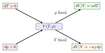
图 1:\(\alpha\) 与 \(\kappa_T\) 是同一个状态函数 \(V(T,p)\) 沿两条不同受约束方向的斜率。
1.2 Isothermal 与 isentropic compression 不同
定义
\[\kappa_S\equiv-\frac{1}{V}\left(\frac{\partial V}{\partial p}\right)_S.\]
绝热可逆压缩使普通材料升温,升温造成额外膨胀趋势,因此相同 \(dp>0\) 下体积减小通常少于恒温情形,即 \(\kappa_S<\kappa_T\)。
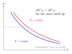
图 2:普通气体的 isentrope 比 isotherm 更陡,对应 \(\kappa_S<\kappa_T\)。
Worked Example 1 — 温度与压强共同改变体积
已知: 液体样品 \(V=1.000\ \mathrm L\),在小范围内 \(\alpha=2.10\times10^{-4}\ \mathrm{K^{-1}}\)、\(\kappa_T=4.60\times10^{-10}\ \mathrm{Pa^{-1}}\);同时 \(\Delta T=+10.0\ \mathrm K\)、\(\Delta p=+5.00\ \mathrm{MPa}\)。
系统与符号: 固定质量单相液体,体积增加为正。
模型理由: 给定变化范围内把 response functions 视为常量,保留一阶项。
\[\frac{\Delta V}{V}\approx\alpha\Delta T-\kappa_T\Delta p =2.10\times10^{-3}-2.30\times10^{-3} =-2.00\times10^{-4}.\]
\[\boxed{\Delta V=-0.200\ \mathrm{mL},\qquad V_f=999.800\ \mathrm{mL}.}\]
检查: 两项均无量纲;加热膨胀和加压压缩方向相反,后者略占优势。若接近沸点或临界点,系数变化显著,常量近似不可用。
Knowledge 2 — Thermodynamic identities among response functions / 响应函数间的热力学恒等式
Knowledge ID: P03-U05-L02-K02
2.1 \(C_p-C_V\) 不是独立参数
由 \(dS\) 在 \((T,V)\) 与 \((T,p)\) 表示下配合 Maxwell relation,可得
\[\boxed{C_p-C_V=TV\frac{\alpha^2}{\kappa_T}.}\]
对稳定普通物质 \(T>0,V>0,\kappa_T>0\),因此 \(C_p\ge C_V\)。等号可能在 \(\alpha=0\) 的特殊温度成立;并非所有固体都严格相等。
另一组重要关系为
\[\boxed{\frac{\kappa_T}{\kappa_S}=\frac{C_p}{C_V},}\]
以及
\[\left(\frac{\partial p}{\partial T}\right)_V=\frac{\alpha}{\kappa_T}.\]
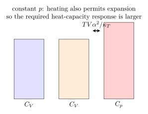
图 3:恒压加热相较恒容加热多出与 thermoelastic coupling 有关的响应;柱高为示意。
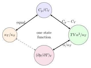
图 4:响应函数由共同势函数产生,测得其中若干项就能交叉核验其余项。
Worked Example 2 — 由 expansivity 与 compressibility 求 \(c_p-c_V\)
已知: 一摩尔流体在 \(T=300\ \mathrm K\) 时 \(V_m=2.50\times10^{-2}\ \mathrm{m^3\,mol^{-1}}\)、\(\alpha=3.40\times10^{-3}\ \mathrm{K^{-1}}\)、\(\kappa_T=1.00\times10^{-5}\ \mathrm{Pa^{-1}}\),且 \(c_V=20.8\ \mathrm{J\,mol^{-1}K^{-1}}\)。
模型: 稳定单相、响应函数在该点有定义。
\[c_p-c_V=TV_m\frac{\alpha^2}{\kappa_T} =300(2.50\times10^{-2})\frac{(3.40\times10^{-3})^2}{1.00\times10^{-5}} =8.67\ \mathrm{J\,mol^{-1}K^{-1}}.\]
\[\boxed{c_p=29.5\ \mathrm{J\,mol^{-1}K^{-1}}.}\]
检查: \(\mathrm{K\,m^3\,mol^{-1}\,K^{-2}Pa=J\,mol^{-1}K^{-1}}\);结果 \(c_p>c_V>0\),与稳定性一致。这里的数据只定义一个局部状态点,不应被误认作特定真实气体的精确常数。
Knowledge 3 — Stability and convexity conditions / 稳定性与凸性条件
Knowledge ID: P03-U05-L02-K03
3.1 稳定平衡要求小涨落提高相应势
固定 \(S,V,N\) 时,稳定态是 \(U\) 的局部最小;对 energy representation,\(U(S,V,N)\) 对 extensive variables 应为 convex。两个直接曲率为
\[\left(\frac{\partial^2U}{\partial S^2}\right)_V =\left(\frac{\partial T}{\partial S}\right)_V =\frac{T}{C_V}>0,\]
\[\left(\frac{\partial^2F}{\partial V^2}\right)_T =-\left(\frac{\partial p}{\partial V}\right)_T =\frac{1}{V\kappa_T}>0.\]
所以普通无约束稳定相要求 \(C_V>0\) 与 \(\kappa_T>0\)。相反,\(G(T,p)\) 对 intensive natural variables 是 concave:
\[\left(\frac{\partial^2G}{\partial T^2}\right)_p=-\frac{C_p}{T}<0, \qquad \left(\frac{\partial^2G}{\partial p^2}\right)_T=-V\kappa_T<0.\]
“所有势都必须凸”是错误说法;曲率方向取决于变量是 extensive 还是 intensive。
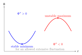
图 5:对允许的 extensive fluctuation,正曲率给 restoring tendency;负曲率会放大涨落。
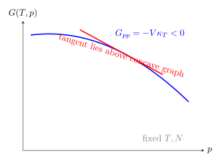
图 6:同一稳定性在 Gibbs representation 中表现为对 pressure 的 concavity,而非 minimum along \(p\)。
3.2 Spinodal 是局部稳定性丧失的边界
在 van der Waals-like subcritical isotherm 的中间支路,\((\partial p/\partial V)_T>0\),因此 \(\kappa_T<0\)。不受外部反馈约束的均匀系统会分离成两相;端点满足 \((\partial p/\partial V)_T=0\),response diverges,称为 spinodal boundary。共存线与 spinodal 不同:前者是全局自由能相等,后者是局部曲率为零。
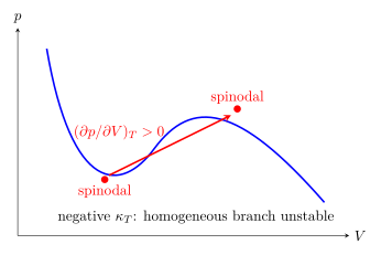
图 7:subcritical loop 的正斜率段对应 negative isothermal compressibility;曲线为示意,不作为具体 equation of state。
Worked Example 3 — 用压缩率识别机械不稳定支路
已知: 某模型 isotherm 在一点有 \(V=1.00\times10^{-3}\ \mathrm{m^3}\) 与 \((\partial p/\partial V)_T=+5.00\times10^{10}\ \mathrm{Pa\,m^{-3}}\)。
系统: 无外部反馈约束的均匀单相候选态,温度固定。
判据: 稳定机械响应要求 \(\kappa_T>0\)。
\[\kappa_T=-\frac{1}{V}\left(\frac{\partial V}{\partial p}\right)_T =-\frac{1}{(1.00\times10^{-3})(5.00\times10^{10})} =-2.00\times10^{-8}\ \mathrm{Pa^{-1}}.\]
\[\boxed{\kappa_T<0:\ \text{the homogeneous branch is mechanically unstable}.}\]
检查: 单位为 \(\mathrm{Pa^{-1}}\);增加压力反而预测体积增加,涨落不会被恢复。实际平衡将由相分离/common tangent 替代,而不是沿该支路持续变化。
Knowledge 4 — Joule and Joule–Thomson processes / 焦耳与焦耳—汤姆孙过程
Knowledge ID: P03-U05-L02-K04
4.1 Joule free expansion:封闭系统、\(U\) 守恒
气体向真空自由膨胀;若外壁绝热且刚性,则 \(Q=0\)、外界压力为零、总边界功为零,所以 \(\Delta U=0\)。把 \(U\) 写成 \(T,V\):
\[dU=C_V\,dT+\left[T\left(\frac{\partial p}{\partial T}\right)_V-p\right]dV.\]
因此 Joule coefficient 为
\[\eta_J\equiv\left(\frac{\partial T}{\partial V}\right)_U =\frac{p-T(\partial p/\partial T)_V}{C_V}.\]
理想气体 \(p=T(\partial p/\partial T)_V\),故 \(\eta_J=0\);真实气体可升温或降温。过程本身不可逆,不能沿过程写 \(\delta Q=T\,dS\)。
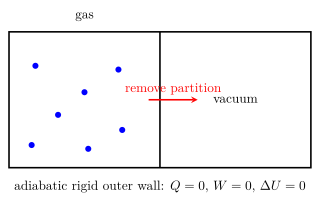
图 8:Joule expansion 的系统边界包住整个刚性容器;内部隔板移动不是对外边界功。
4.2 Joule–Thomson throttling:稳流控制体、\(H\) 守恒
流体通过 porous plug、valve 或 capillary,从高压侧稳流到低压侧。若控制体绝热、无轴功且动能/重力势能变化可忽略,steady-flow energy equation 给 \(h_1=h_2\)。定义
\[\boxed{\mu_{JT}\equiv\left(\frac{\partial T}{\partial p}\right)_H =\frac{T(\partial V/\partial T)_p-V}{C_p} =\frac{V(\alpha T-1)}{C_p}.}\]
压力下降 \(\Delta p<0\):若 \(\mu_{JT}>0\),则 \(\Delta T<0\)(cooling);若 \(\mu_{JT}<0\),则 heating。理想气体 \(\alpha=1/T\),所以 \(\mu_{JT}=0\)。\(\mu_{JT}=0\) 的状态构成 inversion curve,不是一条所有气体共用的常数温度。
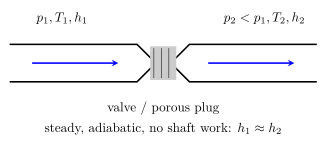
图 9:节流是开放控制体的稳流过程,不能用自由膨胀的封闭系统 \(U\) 守恒替代。
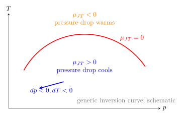
图 10:inversion curve 分隔节流冷却与升温区域;具体形状依赖 equation of state。
Worked Example 4 — 由 \(\alpha\) 判断节流温变
已知: 某真实气体在入口附近 \(T=300\ \mathrm K\)、\(V_m=2.40\times10^{-2}\ \mathrm{m^3\,mol^{-1}}\)、\(c_p=29.1\ \mathrm{J\,mol^{-1}K^{-1}}\)、\(\alpha=3.340\times10^{-3}\ \mathrm{K^{-1}}\)。节流压降 \(\Delta p=-2.00\ \mathrm{MPa}\)。
系统与方向: 稳态绝热阀控制体,忽略速度和高度变化;压力降低为负。
模型理由: 在小压降范围把 \(\mu_{JT}\) 视为常量。
\[\alpha T-1=(3.340\times10^{-3})(300)-1=2.00\times10^{-3},\]
\[\mu_{JT}=\frac{V_m(\alpha T-1)}{c_p} =1.65\times10^{-6}\ \mathrm{K\,Pa^{-1}} =1.65\ \mathrm{K\,MPa^{-1}}.\]
\[\boxed{\Delta T\approx\mu_{JT}\Delta p=(1.65)(-2.00)=-3.30\ \mathrm K.}\]
检查: \(\mu_{JT}>0\) 且 \(\Delta p<0\),所以 cooling;\(V/c_p\) 给 \(\mathrm{K\,Pa^{-1}}\)。较大压降必须沿等焓线积分,不能把入口导数无限外推。
Lesson synthesis / 全课整合
Response functions 是势函数的二阶信息:它们描述材料在指定 constraint 下对小扰动的斜率。因为所有斜率来自同一 exact state function,\(C_p,C_V,\alpha,\kappa_T,\kappa_S\) 必须满足恒等式;因为稳定态要抵抗涨落,它们的符号和势曲率受到限制。Joule 与 Joule–Thomson experiments 则把这些导数转成可观察温变,但两者的系统边界和守恒量不同。
建模流程: 标出单相状态点 → 写清保持量 → 选择 response definition → 用 Maxwell/链式关系减少未知量 → 检查 \(C>0,\kappa>0\) → 对流动或膨胀先画系统边界 → 确认守恒 \(U\) 还是 \(H\) → 根据导数符号判断温变 → 审核线性范围。
Formula-and-decision table / 公式—决策表
| Task | Relation | Use only when | Key caution |
|---|---|---|---|
| small volume response | \(dV/V=\alpha\,dT-\kappa_T\,dp\) | one smooth phase, small changes | coefficients may vary strongly |
| heat-capacity difference | \(C_p-C_V=TV\alpha^2/\kappa_T\) | simple compressible stable phase | use volumetric \(\alpha\) |
| compressibility ratio | \(\kappa_T/\kappa_S=C_p/C_V\) | equilibrium response functions | all quantities at same state |
| thermal stability | \(C_V>0\) and usually \(C_p>0\) | unconstrained macroscopic equilibrium | exotic constrained systems need care |
| mechanical stability | \(\kappa_T>0\) | homogeneous phase without feedback | spinodal has divergent response |
| Joule response | \(\eta_J=[p-T(\partial p/\partial T)_V]/C_V\) | insulated rigid outer boundary, \(U\) fixed | process is irreversible |
| throttling response | \(\mu_{JT}=V(\alpha T-1)/C_p\) | steady adiabatic throttle, \(H\) fixed | integrate for large pressure drop |
Model boundaries / 模型边界
- Linear response assumes perturbations are small relative to the scale on which coefficients change;临界点附近常失效。
- \(C_p-C_V\) identity assumes simple compressible equilibrium matter;额外 generalized work requires an enlarged response matrix。
- Positivity criteria refer to an unconstrained homogeneous subsystem in the thermodynamic limit;gravity、feedback or finite reservoirs can modify accessible fluctuations。
- A spinodal is a local-stability boundary, while coexistence is determined by global potential comparison;不要把两者画成同一线。
- Joule free expansion conserves \(U\) only for the entire insulated rigid container;leaks、wall work or internal energy storage alter the conclusion。
- Joule–Thomson is isenthalpic only under steady-flow approximations;large kinetic-energy change、shaft work and heat exchange require the full energy equation。
Misconception clinic / 易错概念诊所
- “压缩率就是 \(dV/dp\)。” 少了归一化和负号;\(\kappa_T=-(1/V)(\partial V/\partial p)_T\)。
- “\(C_p>C_V\) 因为恒压时温度更高。” 比较的是达到同一微小温升所需响应;差值来自 thermoelastic coupling,而不是最终温度不同。
- “稳定势函数对所有变量都必须向上凸。” extensive natural variables 对应 convex,Legendre-transformed intensive variables常对应 concave。
- “负压缩率只是奇怪材料,也能自由稳定。” 对无反馈的均匀宏观相,\(\kappa_T<0\) 表示局部不稳定;受限或主动系统必须另列机制。
- “Joule expansion 与 throttling 都是气体过小孔,所以守恒量相同。” 前者是封闭绝热刚性系统的 \(U\) 守恒,后者是稳流控制体的 \(H\) 守恒。
- “节流一定冷却。” 只有 \(\mu_{JT}>0\) 且压降为负时冷却;跨 inversion curve 会升温。
Practice and retrieval / 练习与检索
1. 定义辨析(K01)
写出 \(\alpha\) 与 \(\kappa_T\) 定义并给出 SI 单位。
Answer
\(\alpha=(1/V)(\partial V/\partial T)_p\),单位 \(\mathrm{K^{-1}}\);\(\kappa_T=-(1/V)(\partial V/\partial p)_T\),单位 \(\mathrm{Pa^{-1}}\)。
2. 线性体积响应(K01)
\(\alpha=1.0\times10^{-4}\ \mathrm{K^{-1}}\),\(\kappa_T=2.0\times10^{-10}\ \mathrm{Pa^{-1}}\)。若升温 \(5.0\ \mathrm K\) 且压力不变,\(\Delta V/V\) 为多少?
Answer
\(\Delta V/V\approx\alpha\Delta T=5.0\times10^{-4}\),即增加 \(0.050\%\)。
3. 热容恒等式(K02)
在什么条件下 \(C_p=C_V\) 可由一般恒等式得到?
Answer
在 \(T,V\) 有限且 \(\kappa_T\) 非奇异时,若 \(\alpha=0\),则 \(C_p-C_V=TV\alpha^2/\kappa_T=0\)。固体“近似相等”不等于定义上恒等。
4. Adiabatic compressibility(K02)
某气体 \(C_p/C_V=1.40\)、\(\kappa_T=1.00\times10^{-5}\ \mathrm{Pa^{-1}}\)。求 \(\kappa_S\)。
Answer
由 \(\kappa_T/\kappa_S=C_p/C_V\),得 \(\kappa_S=7.14\times10^{-6}\ \mathrm{Pa^{-1}}\)。
5. 热稳定性(K03)
若某均匀候选态给 \(C_V<0\),对小能量交换会发生什么?
Answer
因 \(U_{SS}=T/C_V<0\),对应允许 entropy fluctuation 的曲率错误,小涨落不是 restoring;对通常可加和宏观平衡系统该支路不稳定。有限引力系统等非加和例外需另行分析。
6. Mechanical spinodal(K03)
spinodal 点上 \((\partial p/\partial V)_T\) 和 \(\kappa_T\) 分别怎样?
Answer
理想化 spinodal 上 \((\partial p/\partial V)_T=0\),所以 \((\partial V/\partial p)_T\) 与 \(\kappa_T\) 发散;穿过后均匀支路出现 \(\kappa_T<0\)。
7. Joule expansion(K04)
为什么理想气体自由膨胀温度不变,但熵增加?
Answer
绝热刚性容器给 \(\Delta U=0\);理想气体 \(U=U(T)\),故 \(\Delta T=0\)。可访问体积增加使熵增加,过程不可逆;温度不变不等于等熵。
8. Throttling sign(K04)
若 \(\mu_{JT}=-0.40\ \mathrm{K\,MPa^{-1}}\)、\(\Delta p=-5.0\ \mathrm{MPa}\),估计 \(\Delta T\) 并判断方向。
Answer
\(\Delta T\approx\mu_{JT}\Delta p=+2.0\ \mathrm K\),节流后升温,因为系数和压降均为负。
9. Ideal-gas limit(K04)
用 \(\alpha\) 形式证明理想气体 \(\mu_{JT}=0\)。
Answer
理想气体恒压下 \(V\propto T\),所以 \(\alpha=1/T\)。代入 \(\mu_{JT}=V(\alpha T-1)/C_p\) 得零。
10. 数据自洽审计(K01–K04)
某数据库同一状态给 \(C_p<C_V\)、\(\alpha\ne0\)、\(\kappa_T>0\)。在 simple compressible equilibrium 模型下是否可能?
Answer
不可能;\(C_p-C_V=TV\alpha^2/\kappa_T>0\)。应核对 molar/mass basis、线/体膨胀系数、单位、相态、插值范围与是否处于非平衡或约束系统。
Exit ticket / 课末检验
- 给出一套由 \(V(T,p)\)、\(C_p\) 数据计算 \(C_V\) 与 \(\mu_{JT}\) 的流程,并列出两个稳定性检查。
- 画出 Joule free expansion 与 Joule–Thomson throttling 的系统边界,分别写出零项、守恒量和理想气体极限。
References and source notes / 参考资料与来源说明
- MIT OCW 8.333, Statistical Mechanics I, Lecture 1 — response-function definitions、Joule experiment 与 generalized coordinates。
- MIT OCW 3.020, Lecture 2 transcript — compressibility、volumetric expansivity 与 ideal-gas check。
- MIT OCW 3.00, Lecture 23 — Mathematics and Stability — thermodynamic curvature and stability restrictions。
- MIT OCW 10.40, Chemical Engineering Thermodynamics Readings — derivative manipulation、stability criteria、critical states and real-fluid models。
- MIT OCW 5.60, Lecture 4 — Joule–Thomson coefficient、inversion temperature 与 refrigeration interpretation。
- NIST Chemistry WebBook — Thermophysical Properties of Fluid Systems — \(C_p,C_V\)、Joule–Thomson coefficient 与 phase-aware fluid data fields。
- NIST Monograph 168 — Selected Properties of Hydrogen — \(\mu_{JT}\) definition、sign convention、inversion curve and measurement range。
- NIST REFPROP — critically evaluated equations of state and response functions for real fluids。
以上链接均于 2026-08-25 实际打开并核对到具体页面或 PDF。NIST 数据源用于说明字段、单位与真实流体边界,不把数据库值无来源地移植到例题;图示均按本文方程原创。
Source-to-content map
| Source | Used for | Knowledge ID / Section | Model boundary or convention |
|---|---|---|---|
| MIT 8.333 Lecture 1 | heat capacities, compressibilities, Joule expansion | K01, K04 | equilibrium response and ideal-gas example |
| MIT 3.020 Lecture 2 | definitions and unit conventions | K01 | volumetric rather than linear expansivity |
| MIT 3.00 Lecture 23 | curvature and stability | K03 | local single-phase stability |
| MIT 10.40 readings | identities, stability, critical states | K02, K03 | smooth thermodynamic models |
| MIT 5.60 Lecture 4 | throttling and inversion | K04 | steady isenthalpic approximation |
| NIST Fluid WebBook | available measured/calculated response fields | K01, K04 | phase and standard-state metadata |
| NIST Monograph 168 | JT sign and hydrogen inversion data | K04 | substance- and range-specific |
| NIST REFPROP | real-fluid equations and derivatives | K01–K04 | critically evaluated finite validity ranges |
复习与拓展
- 下一课把局部 stability 与全局 phase coexistence 区分,并推导 Clapeyron slope。
- 系综与配分函数会把 \(C_V\) 与能量涨落、compressibility 与粒子数涨落联系起来。
- 临界性将研究 response divergence、critical exponents 与 universality。
- 工程热力学会把 \(\mu_{JT}\) 沿真实等焓线积分,用于 liquefaction and refrigeration cycle design。